This is a fixed-text formatted version of a Jupyter notebook
Try online

You can contribute with your own notebooks in this GitHub repository.
Source files: spectrum_simulation.ipynb | spectrum_simulation.py
Spectrum simulation for CTA
A quick example how to use the functions and classes in gammapy.spectrum in order to simulate and fit spectra.
We will simulate observations for CTA first using a power law model without any background. Then we will add a power law shaped background component. The next part of the tutorial shows how to use user defined models for simulations and fitting.
We will use the following classes:
Setup
Same procedure as in every script …
[1]:
%matplotlib inline
import matplotlib.pyplot as plt
[2]:
import numpy as np
import astropy.units as u
from astropy.coordinates import SkyCoord, Angle
from regions import CircleSkyRegion
from gammapy.spectrum import (
    SpectrumDatasetOnOff,
    SpectrumDataset,
    SpectrumDatasetMaker,
)
from gammapy.modeling import Fit, Parameter
from gammapy.modeling.models import (
    PowerLawSpectralModel,
    SpectralModel,
    SkyModel,
)
from gammapy.irf import load_cta_irfs
from gammapy.data import Observation
from gammapy.maps import MapAxis
Simulation of a single spectrum
To do a simulation, we need to define the observational parameters like the livetime, the offset, the assumed integration radius, the energy range to perform the simulation for and the choice of spectral model. We then use an in-memory observation which is convolved with the IRFs to get the predicted number of counts. This is Poission fluctuated using the fake() to get the simulated counts for each observation.
[3]:
# Define simulation parameters parameters
livetime = 1 * u.h
pointing = SkyCoord(0, 0, unit="deg", frame="galactic")
offset = 0.5 * u.deg
# Reconstructed and true energy axis
energy_axis = MapAxis.from_edges(
    np.logspace(-0.5, 1.0, 10), unit="TeV", name="energy", interp="log"
)
energy_axis_true = MapAxis.from_edges(
    np.logspace(-1.2, 2.0, 31), unit="TeV", name="energy", interp="log"
)

on_region_radius = Angle("0.11 deg")
on_region = CircleSkyRegion(center=pointing, radius=on_region_radius)
[4]:
# Define spectral model - a simple Power Law in this case
model_simu = PowerLawSpectralModel(
    index=3.0,
    amplitude=2.5e-12 * u.Unit("cm-2 s-1 TeV-1"),
    reference=1 * u.TeV,
)
print(model_simu)
# we set the sky model used in the dataset
model = SkyModel(spectral_model=model_simu)
PowerLawSpectralModel

   name     value   error      unit      min max frozen
--------- --------- ----- -------------- --- --- ------
    index 3.000e+00   nan                nan nan  False
amplitude 2.500e-12   nan cm-2 s-1 TeV-1 nan nan  False
reference 1.000e+00   nan            TeV nan nan   True
[5]:
# Load the IRFs
# In this simulation, we use the CTA-1DC irfs shipped with gammapy.
irfs = load_cta_irfs(
    "$GAMMAPY_DATA/cta-1dc/caldb/data/cta/1dc/bcf/South_z20_50h/irf_file.fits"
)
[6]:
obs = Observation.create(pointing=pointing, livetime=livetime, irfs=irfs)
print(obs)
Info for OBS_ID = 1
- Pointing pos: RA 266.40 deg / Dec -28.94 deg
- Livetime duration: 3600.0 s
WARNING: AstropyDeprecationWarning: The truth value of a Quantity is ambiguous. In the future this will raise a ValueError. [astropy.units.quantity]
[7]:
# Make the SpectrumDataset
dataset_empty = SpectrumDataset.create(
    e_reco=energy_axis.edges, e_true=energy_axis_true.edges, region=on_region
)
maker = SpectrumDatasetMaker(selection=["aeff", "edisp", "background"])
dataset = maker.run(dataset_empty, obs)
[8]:
# Set the model on the dataset, and fake
dataset.model = model
dataset.fake(random_state=42)
print(dataset)
SpectrumDataset

    Name                            : 1

    Total counts                    : 16
    Total predicted counts          : nan
    Total background counts         : 22.35

    Effective area min              : 8.16e+04 m2
    Effective area max              : 5.08e+06 m2

    Livetime                        : 3.60e+03 s

    Number of total bins            : 9
    Number of fit bins              : 9

    Fit statistic type              : cash
    Fit statistic value (-2 log(L)) : nan

    Number of parameters            : 0
    Number of free parameters       : 0
You can see that backgound counts are now simulated
OnOff analysis
To do OnOff spectral analysis, which is the usual science case, the standard would be to use SpectrumDatasetOnOff, which uses the acceptance to fake off-counts
[9]:
dataset_onoff = SpectrumDatasetOnOff(
    aeff=dataset.aeff,
    edisp=dataset.edisp,
    models=model,
    livetime=livetime,
    acceptance=1,
    acceptance_off=5,
)
dataset_onoff.fake(background_model=dataset.background)
print(dataset_onoff)
SpectrumDatasetOnOff

    Name                            :

    Total counts                    : 289
    Total predicted counts          : 297.02
    Total off counts                : 123.00

    Total background counts         : 24.60

    Effective area min              : 8.16e+04 m2
    Effective area max              : 5.08e+06 m2

    Livetime                        : 1.00e+00 h

    Number of total bins            : 9
    Number of fit bins              : 9

    Fit statistic type              : wstat
    Fit statistic value (-2 log(L)) : 10.22

    Number of parameters            : 3
    Number of free parameters       : 2

    Model type                      : SkyModels
    Acceptance mean:                : 1.0
You can see that off counts are now simulated as well. We now simulate several spectra using the same set of observation conditions.
[10]:
%%time

n_obs = 100
datasets = []

for idx in range(n_obs):
    dataset_onoff.fake(random_state=idx, background_model=dataset.background)
    dataset_onoff.name = f"obs_{idx}"
    datasets.append(dataset_onoff.copy())
CPU times: user 220 ms, sys: 4.87 ms, total: 225 ms
Wall time: 228 ms
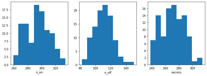
Before moving on to the fit let’s have a look at the simulated observations.
[11]:
n_on = [dataset.counts.data.sum() for dataset in datasets]
n_off = [dataset.counts_off.data.sum() for dataset in datasets]
excess = [dataset.excess.data.sum() for dataset in datasets]

fix, axes = plt.subplots(1, 3, figsize=(12, 4))
axes[0].hist(n_on)
axes[0].set_xlabel("n_on")
axes[1].hist(n_off)
axes[1].set_xlabel("n_off")
axes[2].hist(excess)
axes[2].set_xlabel("excess");
Now, we fit each simulated spectrum individually
[12]:
%%time
results = []
for dataset in datasets:
    dataset.models = model.copy()
    fit = Fit([dataset])
    result = fit.optimize()
    results.append(
        {
            "index": result.parameters["index"].value,
            "amplitude": result.parameters["amplitude"].value,
        }
    )
CPU times: user 4.6 s, sys: 43.3 ms, total: 4.65 s
Wall time: 4.72 s
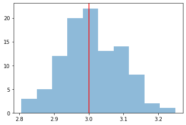
We take a look at the distribution of the fitted indices. This matches very well with the spectrum that we initially injected, index=2.1
[13]:
index = np.array([_["index"] for _ in results])
plt.hist(index, bins=10, alpha=0.5)
plt.axvline(x=model_simu.parameters["index"].value, color="red")
print(f"index: {index.mean()} += {index.std()}")
index: 3.008268371884822 += 0.08582628065923613
Adding a user defined model
Many spectral models in gammapy are subclasses of gammapy.modeling.models.SpectralModel. The list of available models is shown below.
[14]:
SpectralModel.__subclasses__()
[14]:
[gammapy.modeling.models.spectral.ConstantSpectralModel,
 gammapy.modeling.models.spectral.CompoundSpectralModel,
 gammapy.modeling.models.spectral.PowerLawSpectralModel,
 gammapy.modeling.models.spectral.PowerLaw2SpectralModel,
 gammapy.modeling.models.spectral.ExpCutoffPowerLawSpectralModel,
 gammapy.modeling.models.spectral.ExpCutoffPowerLaw3FGLSpectralModel,
 gammapy.modeling.models.spectral.SuperExpCutoffPowerLaw3FGLSpectralModel,
 gammapy.modeling.models.spectral.SuperExpCutoffPowerLaw4FGLSpectralModel,
 gammapy.modeling.models.spectral.LogParabolaSpectralModel,
 gammapy.modeling.models.spectral.TemplateSpectralModel,
 gammapy.modeling.models.spectral.ScaleSpectralModel,
 gammapy.modeling.models.spectral.AbsorbedSpectralModel,
 gammapy.modeling.models.spectral.NaimaSpectralModel,
 gammapy.modeling.models.spectral.GaussianSpectralModel,
 gammapy.modeling.models.spectral_cosmic_ray._LogGaussianSpectralModel,
 gammapy.modeling.models.spectral_crab.MeyerCrabSpectralModel]
This section shows how to add a user defined spectral model.
To do that you need to subclass SpectralModel. All SpectralModel subclasses need to have an __init__ function, which sets up the Parameters of the model and a static function called evaluate where the mathematical expression for the model is defined.
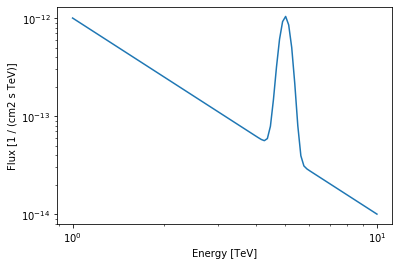
As an example we will use a PowerLawSpectralModel plus a Gaussian (with fixed width).
[15]:
class UserModel(SpectralModel):
    index = Parameter("index", 2, min=0)
    amplitude = Parameter("amplitude", "1e-12 cm-2 s-1 TeV-1", min=0)
    reference = Parameter("reference", "1 TeV", frozen=True)
    mean = Parameter("mean", "1 TeV", min=0)
    width = Parameter("width", "0.1 TeV", min=0, frozen=True)

    @staticmethod
    def evaluate(energy, index, amplitude, reference, mean, width):
        pwl = PowerLawSpectralModel.evaluate(
            energy=energy,
            index=index,
            amplitude=amplitude,
            reference=reference,
        )
        gauss = amplitude * np.exp(-((energy - mean) ** 2) / (2 * width ** 2))
        return pwl + gauss
[16]:
model = UserModel(
    index=2,
    amplitude=1e-12 * u.Unit("cm-2 s-1 TeV-1"),
    reference=1 * u.TeV,
    mean=5 * u.TeV,
    width=0.2 * u.TeV,
)
print(model)
UserModel

   name     value   error      unit         min    max frozen
--------- --------- ----- -------------- --------- --- ------
    index 2.000e+00   nan                0.000e+00 nan  False
amplitude 1.000e-12   nan cm-2 s-1 TeV-1 0.000e+00 nan  False
reference 1.000e+00   nan            TeV       nan nan   True
     mean 5.000e+00   nan            TeV 0.000e+00 nan  False
    width 2.000e-01   nan            TeV 0.000e+00 nan   True
[17]:
energy_range = [1, 10] * u.TeV
model.plot(energy_range=energy_range);
Exercises
Change the observation time to something longer or shorter. Does the observation and spectrum results change as you expected?
Change the spectral model, e.g. add a cutoff at 5 TeV, or put a steep-spectrum source with spectral index of 4.0
Simulate spectra with the spectral model we just defined. How much observation duration do you need to get back the injected parameters?
What next?
In this tutorial we simulated and analysed the spectrum of source using CTA prod 2 IRFs.
If you’d like to go further, please see the other tutorial notebooks.
[ ]: