This is a fixed-text formatted version of a Jupyter notebook

Try online
You can contribute with your own notebooks in this GitHub repository.
Source files: spectrum_analysis.ipynb | spectrum_analysis.py

Spectral analysis with Gammapy¶

Introduction¶

This notebook explains in detail how to use the classes in gammapy.spectrum and related ones.

Based on a datasets of 4 Crab observations with H.E.S.S. we will perform a full region based spectral analysis, i.e. extracting source and background counts from certain regions, and fitting them using the forward-folding approach. We will use the following classes

Data handling:

To extract the 1-dim spectral information:

To perform the joint fit:

To compute flux points (a.k.a. “SED” = “spectral energy distribution”)

Feedback welcome!

Setup¶

As usual, we’ll start with some setup …

[1]:

%matplotlib inline
import matplotlib.pyplot as plt

[2]:

# Check package versions
import gammapy
import numpy as np
import astropy
import regions

print("gammapy:", gammapy.__version__)
print("numpy:", np.__version__)
print("astropy", astropy.__version__)
print("regions", regions.__version__)

gammapy: 0.15
numpy: 1.17.3
astropy 3.2.3
regions 0.4

[3]:

from pathlib import Path
import astropy.units as u
from astropy.coordinates import SkyCoord, Angle
from regions import CircleSkyRegion
from gammapy.maps import Map
from gammapy.modeling import Fit, Datasets
from gammapy.data import DataStore
from gammapy.modeling.models import (
    PowerLawSpectralModel,
    create_crab_spectral_model,
    SkyModel,
)
from gammapy.cube import SafeMaskMaker
from gammapy.spectrum import (
    SpectrumDatasetMaker,
    SpectrumDatasetOnOff,
    SpectrumDataset,
    FluxPointsEstimator,
    FluxPointsDataset,
    ReflectedRegionsBackgroundMaker,
    plot_spectrum_datasets_off_regions,
)

Load Data¶

First, we select and load some H.E.S.S. observations of the Crab nebula (simulated events for now).

We will access the events, effective area, energy dispersion, livetime and PSF for containement correction.

[4]:

datastore = DataStore.from_dir("$GAMMAPY_DATA/hess-dl3-dr1/")
obs_ids = [23523, 23526, 23559, 23592]
observations = datastore.get_observations(obs_ids)

Define Target Region¶

The next step is to define a signal extraction region, also known as on region. In the simplest case this is just a CircleSkyRegion, but here we will use the Target class in gammapy that is useful for book-keeping if you run several analysis in a script.

[5]:

target_position = SkyCoord(ra=83.63, dec=22.01, unit="deg", frame="icrs")
on_region_radius = Angle("0.11 deg")
on_region = CircleSkyRegion(center=target_position, radius=on_region_radius)

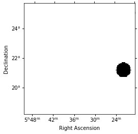
Create exclusion mask¶

We will use the reflected regions method to place off regions to estimate the background level in the on region. To make sure the off regions don’t contain gamma-ray emission, we create an exclusion mask.

Using http://gamma-sky.net/ we find that there’s only one known gamma-ray source near the Crab nebula: the AGN called RGB J0521+212 at GLON = 183.604 deg and GLAT = -8.708 deg.

[6]:

exclusion_region = CircleSkyRegion(
    center=SkyCoord(183.604, -8.708, unit="deg", frame="galactic"),
    radius=0.5 * u.deg,
)

skydir = target_position.galactic
exclusion_mask = Map.create(
    npix=(150, 150), binsz=0.05, skydir=skydir, proj="TAN", coordsys="CEL"
)

mask = exclusion_mask.geom.region_mask([exclusion_region], inside=False)
exclusion_mask.data = mask
exclusion_mask.plot();

../_images/notebooks_spectrum_analysis_12_0.png

Run data reduction chain¶

We begin with the configuration of the maker classes:

[7]:

e_reco = np.logspace(-1, np.log10(40), 40) * u.TeV
e_true = np.logspace(np.log10(0.05), 2, 200) * u.TeV
dataset_empty = SpectrumDataset.create(
    e_reco=e_reco, e_true=e_true, region=on_region
)

[8]:

dataset_maker = SpectrumDatasetMaker(
    containment_correction=False, selection=["counts", "aeff", "edisp"]
)
bkg_maker = ReflectedRegionsBackgroundMaker(exclusion_mask=exclusion_mask)
safe_mask_masker = SafeMaskMaker(methods=["aeff-max"], aeff_percent=10)

[9]:

%%time
datasets = []

for observation in observations:
    dataset = dataset_maker.run(dataset_empty, observation)
    dataset_on_off = bkg_maker.run(dataset, observation)
    dataset_on_off = safe_mask_masker.run(dataset_on_off, observation)
    datasets.append(dataset_on_off)

CPU times: user 2.57 s, sys: 84.4 ms, total: 2.66 s
Wall time: 2.68 s

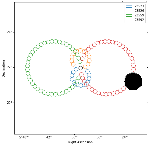
Plot off regions¶

[10]:

plt.figure(figsize=(8, 8))
_, ax, _ = exclusion_mask.plot()
on_region.to_pixel(ax.wcs).plot(ax=ax, edgecolor="k")
plot_spectrum_datasets_off_regions(ax=ax, datasets=datasets)

../_images/notebooks_spectrum_analysis_18_0.png

Source statistic¶

Next we’re going to look at the overall source statistics in our signal region.

[11]:

datasets_all = Datasets(datasets)

[12]:

info_table = datasets_all.info_table(cumulative=True)

[13]:

info_table

[13]:

Table length=4

name	livetime	a_on	n_on	n_off	a_off	alpha	background	excess	significance	background_rate	gamma_rate
	s									1 / s	1 / s
str5	float64	float64	int64	int64	float64	float64	float64	float64	float64	float64	float64
23523	1581.7367584109306	1.0	172	162	12.0	0.08333333333333333	13.5	158.5	21.108139320737838	0.008534922090046502	0.10020630750165709
23523	3154.4234824180603	1.0	365	384	12.0	0.08333333333333333	31.999999999999993	333.0	29.933816690058016	0.01014448446074527	0.10556604141963048
23523	4732.546999931335	1.0	512	790	18.853317811408616	0.05304106205619018	41.90243902439024	470.09756097560984	37.37127329585745	0.008854098865790071	0.09933288797394521
23523	6313.811640620232	1.0	636	1173	22.325282717179665	0.0447922659107239	52.54132791327913	583.4586720867208	41.98855362476707	0.008321649568265832	0.09240989521021017

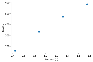
[14]:

plt.plot(
    info_table["livetime"].to("h"), info_table["excess"], marker="o", ls="none"
)
plt.xlabel("Livetime [h]")
plt.ylabel("Excess");

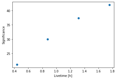
../_images/notebooks_spectrum_analysis_23_0.png

[15]:

plt.plot(
    info_table["livetime"].to("h"),
    info_table["significance"],
    marker="o",
    ls="none",
)
plt.xlabel("Livetime [h]")
plt.ylabel("Significance");

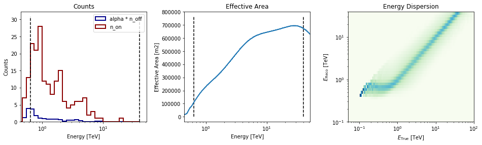
../_images/notebooks_spectrum_analysis_24_0.png

[16]:

datasets[0].peek()

../_images/notebooks_spectrum_analysis_25_0.png

Finally you can write the extrated datasets to disk using the OGIP format (PHA, ARF, RMF, BKG, see here for details):

[17]:

path = Path("spectrum_analysis")
path.mkdir(exist_ok=True)

[18]:

for dataset in datasets:
    dataset.to_ogip_files(outdir=path, overwrite=True)

If you want to read back the datasets from disk you can use:

[19]:

datasets = []
for obs_id in obs_ids:
    filename = path / f"pha_obs{obs_id}.fits"
    datasets.append(SpectrumDatasetOnOff.from_ogip_files(filename))

Fit spectrum¶

Now we’ll fit a global model to the spectrum. First we do a joint likelihood fit to all observations. If you want to stack the observations see below. We will also produce a debug plot in order to show how the global fit matches one of the individual observations.

[20]:

spectral_model = PowerLawSpectralModel(
    index=2, amplitude=2e-11 * u.Unit("cm-2 s-1 TeV-1"), reference=1 * u.TeV
)
model = SkyModel(spectral_model=spectral_model)

for dataset in datasets:
    dataset.models = model

fit_joint = Fit(datasets)
result_joint = fit_joint.run()

# we make a copy here to compare it later
model_best_joint = model.copy()
model_best_joint.spectral_model.parameters.covariance = (
    result_joint.parameters.covariance
)

[21]:

print(result_joint)

OptimizeResult

        backend    : minuit
        method     : minuit
        success    : True
        message    : Optimization terminated successfully.
        nfev       : 48
        total stat : 121.98

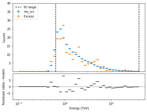
[22]:

plt.figure(figsize=(8, 6))
ax_spectrum, ax_residual = datasets[0].plot_fit()
ax_spectrum.set_ylim(0.1, 40)

[22]:

(0.1, 40)

../_images/notebooks_spectrum_analysis_34_1.png

Compute Flux Points¶

To round up our analysis we can compute flux points by fitting the norm of the global model in energy bands. We’ll use a fixed energy binning for now:

[23]:

e_min, e_max = 0.7, 30
e_edges = np.logspace(np.log10(e_min), np.log10(e_max), 11) * u.TeV

Now we create an instance of the gammapy.spectrum.FluxPointsEstimator, by passing the dataset and the energy binning:

[24]:

fpe = FluxPointsEstimator(datasets=datasets, e_edges=e_edges)
flux_points = fpe.run()

Here is a the table of the resulting flux points:

[25]:

flux_points.table_formatted

[25]:

Table length=10

e_ref	e_min	e_max	ref_dnde	ref_flux	ref_eflux	ref_e2dnde	norm	stat	norm_err	counts [4]	norm_errp	norm_errn	norm_ul	sqrt_ts	ts	norm_scan [11]	stat_scan [11]	dnde	dnde_ul	dnde_err	dnde_errp	dnde_errn
TeV	TeV	TeV	1 / (cm2 s TeV)	1 / (cm2 s)	TeV / (cm2 s)	TeV / (cm2 s)												1 / (cm2 s TeV)	1 / (cm2 s TeV)	1 / (cm2 s TeV)	1 / (cm2 s TeV)	1 / (cm2 s TeV)
float64	float64	float64	float64	float64	float64	float64	float64	float64	float64	int64	float64	float64	float64	float64	float64	float64	float64	float64	float64	float64	float64	float64
0.859	0.737	1.002	4.041e-11	1.078e-11	9.179e-12	2.983e-11	0.968	18.393	0.087	49 .. 31	0.089	0.084	1.151	20.687	427.949	0.200 .. 5.000	188.767 .. 680.271	3.912e-11	4.653e-11	3.501e-12	3.606e-12	3.398e-12
1.261	1.002	1.588	1.489e-11	8.853e-12	1.095e-11	2.369e-11	0.973	12.648	0.091	31 .. 36	0.094	0.088	1.165	20.512	420.723	0.200 .. 5.000	172.542 .. 614.494	1.448e-11	1.734e-11	1.350e-12	1.392e-12	1.310e-12
1.852	1.588	2.160	5.484e-12	3.152e-12	5.788e-12	1.881e-11	1.196	9.917	0.149	27 .. 12	0.156	0.143	1.519	15.287	233.701	0.200 .. 5.000	115.920 .. 242.783	6.560e-12	8.330e-12	8.191e-13	8.528e-13	7.862e-13
2.518	2.160	2.936	2.467e-12	1.928e-12	4.813e-12	1.564e-11	1.249	9.185	0.177	10 .. 11	0.185	0.168	1.635	13.945	194.460	0.200 .. 5.000	96.429 .. 175.789	3.080e-12	4.032e-12	4.354e-13	4.566e-13	4.150e-13
3.697	2.936	4.656	9.086e-13	1.584e-12	5.743e-12	1.242e-11	0.940	14.937	0.158	17 .. 11	0.167	0.150	1.291	10.703	114.552	0.200 .. 5.000	60.543 .. 213.272	8.543e-13	1.173e-12	1.439e-13	1.519e-13	1.362e-13
5.429	4.656	6.330	3.347e-13	5.639e-13	3.035e-12	9.864e-12	1.134	8.760	0.265	9 .. 5	0.286	0.246	1.746	8.141	66.270	0.200 .. 5.000	38.226 .. 81.164	3.794e-13	5.845e-13	8.885e-14	9.562e-14	8.236e-14
7.971	6.330	10.037	1.233e-13	4.632e-13	3.621e-12	7.833e-12	1.040	12.425	0.274	5 .. 4	0.297	0.253	1.681	6.855	46.987	0.200 .. 5.000	32.858 .. 80.471	1.282e-13	2.072e-13	3.382e-14	3.663e-14	3.114e-14
11.703	10.037	13.647	4.541e-14	1.649e-13	1.914e-12	6.220e-12	0.901	10.499	0.429	0 .. 1	0.490	0.373	2.006	3.369	11.351	0.200 .. 5.000	15.510 .. 38.333	4.091e-14	9.110e-14	1.950e-14	2.226e-14	1.696e-14
17.183	13.647	21.636	1.673e-14	1.355e-13	2.284e-12	4.939e-12	0.310	7.211	0.281	1 .. 0	0.357	0.310	1.184	0.950	0.903	0.200 .. 5.000	7.394 .. 43.010	5.186e-15	1.980e-14	4.704e-15	5.976e-15	5.186e-15
25.229	21.636	29.419	6.162e-15	4.825e-14	1.207e-12	3.922e-12	0.000	0.524	0.001	0 .. 0	0.278	0.000	1.110	0.003	0.000	0.200 .. 5.000	1.244 .. 18.536	1.100e-20	6.842e-15	8.675e-18	1.710e-15	1.100e-20

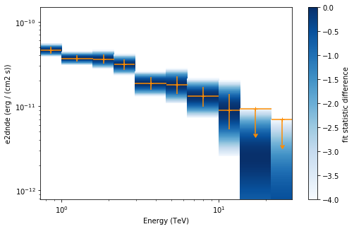
Now we plot the flux points and their likelihood profiles. For the plotting of upper limits we choose a threshold of TS < 4.

[26]:

plt.figure(figsize=(8, 5))
flux_points.table["is_ul"] = flux_points.table["ts"] < 4
ax = flux_points.plot(
    energy_power=2, flux_unit="erg-1 cm-2 s-1", color="darkorange"
)
flux_points.to_sed_type("e2dnde").plot_ts_profiles(ax=ax)

[26]:

<matplotlib.axes._subplots.AxesSubplot at 0x11de538d0>

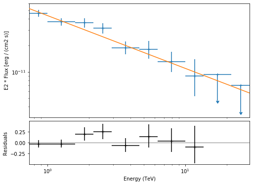
../_images/notebooks_spectrum_analysis_42_1.png

The final plot with the best fit model, flux points and residuals can be quickly made like this:

[27]:

flux_points_dataset = FluxPointsDataset(
    data=flux_points, models=model_best_joint
)

[28]:

plt.figure(figsize=(8, 6))
flux_points_dataset.peek();

../_images/notebooks_spectrum_analysis_45_0.png

Stack observations¶

And alternative approach to fitting the spectrum is stacking all observations first and the fitting a model. For this we first stack the individual datasets:

[29]:

dataset_stacked = Datasets(datasets).stack_reduce()

Again we set the model on the dataset we would like to fit (in this case it’s only a single one) and pass it to the gammapy.modeling.Fit object:

[30]:

dataset_stacked.model = model
stacked_fit = Fit([dataset_stacked])
result_stacked = stacked_fit.run()

# make a copy to compare later
model_best_stacked = model.copy()
model_best_stacked.spectral_model.parameters.covariance = (
    result_stacked.parameters.covariance
)

[31]:

print(result_stacked)

OptimizeResult

        backend    : minuit
        method     : minuit
        success    : True
        message    : Optimization terminated successfully.
        nfev       : 31
        total stat : 34.28

[32]:

model_best_joint.parameters.to_table()

[32]:

Table length=3

name	value	error	unit	min	max	frozen
str9	float64	float64	str14	float64	float64	bool
index	2.600e+00	5.889e-02		nan	nan	False
amplitude	2.723e-11	1.240e-12	cm-2 s-1 TeV-1	nan	nan	False
reference	1.000e+00	0.000e+00	TeV	nan	nan	True

[33]:

model_best_stacked.parameters.to_table()

[33]:

Table length=3

name	value	error	unit	min	max	frozen
str9	float64	float64	str14	float64	float64	bool
index	2.600e+00	6.334e-02		nan	nan	False
amplitude	2.723e-11	1.108e-12	cm-2 s-1 TeV-1	nan	nan	False
reference	1.000e+00	0.000e+00	TeV	nan	nan	True

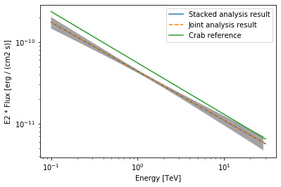
Finally, we compare the results of our stacked analysis to a previously published Crab Nebula Spectrum for reference. This is available in gammapy.spectrum.

[34]:

plot_kwargs = {
    "energy_range": [0.1, 30] * u.TeV,
    "energy_power": 2,
    "flux_unit": "erg-1 cm-2 s-1",
}

# plot stacked model
model_best_stacked.spectral_model.plot(
    **plot_kwargs, label="Stacked analysis result"
)
model_best_stacked.spectral_model.plot_error(**plot_kwargs)

# plot joint model
model_best_joint.spectral_model.plot(
    **plot_kwargs, label="Joint analysis result", ls="--"
)
model_best_joint.spectral_model.plot_error(**plot_kwargs)

create_crab_spectral_model("hess_pl").plot(
    **plot_kwargs, label="Crab reference"
)
plt.legend()

[34]:

<matplotlib.legend.Legend at 0x11eb813c8>

../_images/notebooks_spectrum_analysis_54_1.png

Exercises¶

Now you have learned the basics of a spectral analysis with Gammapy. To practice you can continue with the following exercises:

Fit a different spectral model to the data. You could try gammapy.modeling.models.ExpCutoffPowerLawSpectralModel or gammapy.modeling.models.LogParabolaSpectralModel.
Compute flux points for the stacked dataset.
Create a gammapy.spectrum.FluxPointsDataset with the flux points you have computed for the stacked dataset and fit the flux points again with obe of the spectral models. How does the result compare to the best fit model, that was directly fitted to the counts data?

[ ]: