Note
Go to the end to download the full example code or to run this example in your browser via Binder
Basic image exploration and fitting#
Detect sources, produce a sky image and a spectrum using CTA 1DC data.
Introduction#
This notebook shows an example how to make a sky image and spectrum for simulated CTA data with Gammapy.
The dataset we will use is three observation runs on the Galactic center. This is a tiny (and thus quick to process and play with and learn) subset of the simulated CTA dataset that was produced for the first data challenge in August 2017.
Setup#
As usual, we’ll start with some setup …
# Configure the logger, so that the spectral analysis
# isn't so chatty about what it's doing.
import logging
import numpy as np
import astropy.units as u
from astropy.coordinates import SkyCoord
from regions import CircleSkyRegion

# %matplotlib inline
import matplotlib.pyplot as plt
from IPython.display import display
from gammapy.data import DataStore
from gammapy.datasets import Datasets, FluxPointsDataset, MapDataset, SpectrumDataset
from gammapy.estimators import FluxPointsEstimator, TSMapEstimator
from gammapy.estimators.utils import find_peaks
from gammapy.makers import (
    MapDatasetMaker,
    ReflectedRegionsBackgroundMaker,
    SafeMaskMaker,
    SpectrumDatasetMaker,
)
from gammapy.maps import MapAxis, RegionGeom, WcsGeom
from gammapy.modeling import Fit
from gammapy.modeling.models import (
    GaussianSpatialModel,
    PowerLawSpectralModel,
    SkyModel,
)
from gammapy.visualization import plot_spectrum_datasets_off_regions

logging.basicConfig()
log = logging.getLogger("gammapy.spectrum")
log.setLevel(logging.ERROR)
Check setup#
from gammapy.utils.check import check_tutorials_setup

check_tutorials_setup()
System:

        python_executable      : /home/runner/work/gammapy-docs/gammapy-docs/gammapy/.tox/build_docs/bin/python
        python_version         : 3.9.16
        machine                : x86_64
        system                 : Linux


Gammapy package:

        version                : 1.0.1
        path                   : /home/runner/work/gammapy-docs/gammapy-docs/gammapy/.tox/build_docs/lib/python3.9/site-packages/gammapy


Other packages:

        numpy                  : 1.24.2
        scipy                  : 1.10.1
        astropy                : 5.2.1
        regions                : 0.7
        click                  : 8.1.3
        yaml                   : 6.0
        IPython                : 8.11.0
        jupyterlab             : not installed
        matplotlib             : 3.7.1
        pandas                 : not installed
        healpy                 : 1.16.2
        iminuit                : 2.21.0
        sherpa                 : 4.15.0
        naima                  : 0.10.0
        emcee                  : 3.1.4
        corner                 : 2.2.1


Gammapy environment variables:

        GAMMAPY_DATA           : /home/runner/work/gammapy-docs/gammapy-docs/gammapy-datasets/1.0.1
Select observations#
A Gammapy analysis usually starts by creating a
DataStore and selecting observations.
This is shown in detail in the other notebook, here we just pick three observations near the galactic center.
data_store = DataStore.from_dir("$GAMMAPY_DATA/cta-1dc/index/gps")

# Just as a reminder: this is how to select observations
# from astropy.coordinates import SkyCoord
# table = data_store.obs_table
# pos_obs = SkyCoord(table['GLON_PNT'], table['GLAT_PNT'], frame='galactic', unit='deg')
# pos_target = SkyCoord(0, 0, frame='galactic', unit='deg')
# offset = pos_target.separation(pos_obs).deg
# mask = (1 < offset) & (offset < 2)
# table = table[mask]
# table.show_in_browser(jsviewer=True)

obs_id = [110380, 111140, 111159]
observations = data_store.get_observations(obs_id)

obs_cols = ["OBS_ID", "GLON_PNT", "GLAT_PNT", "LIVETIME"]
display(data_store.obs_table.select_obs_id(obs_id)[obs_cols])
OBS_ID      GLON_PNT           GLAT_PNT      LIVETIME
              deg                deg            s
------ ------------------ ------------------ --------
110380  359.9999912037958 -1.299995937905366   1764.0
111140  358.4999833830074 1.3000020211954284   1764.0
111159 1.5000056568267741  1.299940468335294   1764.0
Make sky images#
Define map geometry#
Select the target position and define an ON region for the spectral analysis
axis = MapAxis.from_edges(
    np.logspace(-1.0, 1.0, 10), unit="TeV", name="energy", interp="log"
)
geom = WcsGeom.create(
    skydir=(0, 0), npix=(500, 400), binsz=0.02, frame="galactic", axes=[axis]
)
print(geom)
WcsGeom

        axes       : ['lon', 'lat', 'energy']
        shape      : (500, 400, 9)
        ndim       : 3
        frame      : galactic
        projection : CAR
        center     : 0.0 deg, 0.0 deg
        width      : 10.0 deg x 8.0 deg
        wcs ref    : 0.0 deg, 0.0 deg
Compute images#
stacked = MapDataset.create(geom=geom)
stacked.edisp = None
maker = MapDatasetMaker(selection=["counts", "background", "exposure", "psf"])
maker_safe_mask = SafeMaskMaker(methods=["offset-max"], offset_max=2.5 * u.deg)

for obs in observations:
    cutout = stacked.cutout(obs.pointing_radec, width="5 deg")
    dataset = maker.run(cutout, obs)
    dataset = maker_safe_mask.run(dataset, obs)
    stacked.stack(dataset)

#
# The maps are cubes, with an energy axis.
# Let's also make some images:
#

dataset_image = stacked.to_image()
geom_image = dataset_image.geoms["geom"]
/home/runner/work/gammapy-docs/gammapy-docs/gammapy/.tox/build_docs/lib/python3.9/site-packages/astropy/units/core.py:2097: UnitsWarning: '1/s/MeV/sr' did not parse as fits unit: Numeric factor not supported by FITS If this is meant to be a custom unit, define it with 'u.def_unit'. To have it recognized inside a file reader or other code, enable it with 'u.add_enabled_units'. For details, see https://docs.astropy.org/en/latest/units/combining_and_defining.html
  warnings.warn(msg, UnitsWarning)
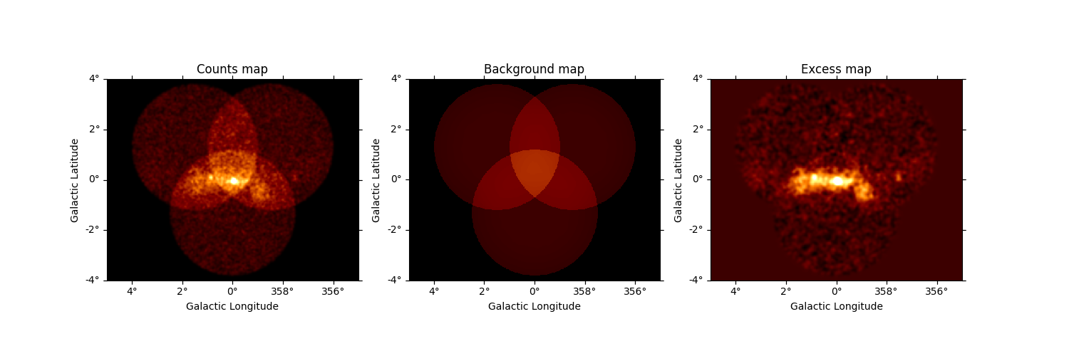
Show images#
Let’s have a quick look at the images we computed …
fig, (ax1, ax2, ax3) = plt.subplots(
    figsize=(15, 5),
    ncols=3,
    subplot_kw={"projection": geom_image.wcs},
    gridspec_kw={"left": 0.1, "right": 0.9},
)

ax1.set_title("Counts map")
dataset_image.counts.smooth(2).plot(ax=ax1, vmax=5)

ax2.set_title("Background map")
dataset_image.background.plot(ax=ax2, vmax=5)

ax3.set_title("Excess map")
dataset_image.excess.smooth(3).plot(ax=ax3, vmax=2)
<WCSAxes: title={'center': 'Excess map'}>
Source Detection#
Use the class TSMapEstimator and function
find_peaks to detect sources on the images.
We search for 0.1 deg sigma gaussian sources in the dataset.
spatial_model = GaussianSpatialModel(sigma="0.05 deg")
spectral_model = PowerLawSpectralModel(index=2)
model = SkyModel(spatial_model=spatial_model, spectral_model=spectral_model)

ts_image_estimator = TSMapEstimator(
    model,
    kernel_width="0.5 deg",
    selection_optional=[],
    downsampling_factor=2,
    sum_over_energy_groups=False,
    energy_edges=[0.1, 10] * u.TeV,
)
images_ts = ts_image_estimator.run(stacked)

sources = find_peaks(
    images_ts["sqrt_ts"],
    threshold=5,
    min_distance="0.2 deg",
)
display(sources)
value   x   y      ra       dec
                  deg       deg
------ --- --- --------- ---------
35.937 252 197 266.42400 -29.00490
17.899 207 202 266.85900 -28.18386
12.762 186 200 267.14365 -27.84496
9.9757 373 205 264.79470 -30.97749
8.6616 306 185 266.01081 -30.05120
8.0451 298 169 266.42267 -30.08192
7.3817 274 217 265.77047 -29.17056
 6.692  90 209 268.07455 -26.10409
5.0221  87 226 267.78333 -25.87897
To get the position of the sources, simply
source_pos = SkyCoord(sources["ra"], sources["dec"])
print(source_pos)
<SkyCoord (ICRS): (ra, dec) in deg
    [(266.42399798, -29.00490483), (266.85900392, -28.18385658),
     (267.14365055, -27.84495923), (264.79469899, -30.97749371),
     (266.01080642, -30.05120198), (266.4226731 , -30.08192101),
     (265.77046935, -29.1705559 ), (268.07454639, -26.10409446),
     (267.78332719, -25.87897418)]>
Plot sources on top of significance sky image
fig, ax = plt.subplots(figsize=(8, 6), subplot_kw={"projection": geom_image.wcs})
images_ts["sqrt_ts"].plot(ax=ax, add_cbar=True)

ax.scatter(
    source_pos.ra.deg,
    source_pos.dec.deg,
    transform=ax.get_transform("icrs"),
    color="none",
    edgecolor="white",
    marker="o",
    s=200,
    lw=1.5,
)
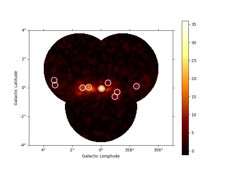
<matplotlib.collections.PathCollection object at 0x7f31816e1700>
Spatial analysis#
See other notebooks for how to run a 3D cube or 2D image based analysis.
Spectrum#
We’ll run a spectral analysis using the classical reflected regions background estimation method, and using the on-off (often called WSTAT) likelihood function.
target_position = SkyCoord(0, 0, unit="deg", frame="galactic")
on_radius = 0.2 * u.deg
on_region = CircleSkyRegion(center=target_position, radius=on_radius)

exclusion_mask = ~geom.to_image().region_mask([on_region])
plt.figure()
exclusion_mask.plot()
<WCSAxes: >
Configure spectral analysis
energy_axis = MapAxis.from_energy_bounds(0.1, 40, 40, unit="TeV", name="energy")
energy_axis_true = MapAxis.from_energy_bounds(
    0.05, 100, 200, unit="TeV", name="energy_true"
)

geom = RegionGeom.create(region=on_region, axes=[energy_axis])
dataset_empty = SpectrumDataset.create(geom=geom, energy_axis_true=energy_axis_true)

dataset_maker = SpectrumDatasetMaker(
    containment_correction=False, selection=["counts", "exposure", "edisp"]
)
bkg_maker = ReflectedRegionsBackgroundMaker(exclusion_mask=exclusion_mask)
safe_mask_masker = SafeMaskMaker(methods=["aeff-max"], aeff_percent=10)
Run data reduction
datasets = Datasets()

for observation in observations:
    dataset = dataset_maker.run(
        dataset_empty.copy(name=f"obs-{observation.obs_id}"), observation
    )
    dataset_on_off = bkg_maker.run(dataset, observation)
    dataset_on_off = safe_mask_masker.run(dataset_on_off, observation)
    datasets.append(dataset_on_off)
/home/runner/work/gammapy-docs/gammapy-docs/gammapy/.tox/build_docs/lib/python3.9/site-packages/gammapy/maps/geom.py:48: RuntimeWarning: invalid value encountered in cast
  p_idx = np.rint(p).astype(int)
/home/runner/work/gammapy-docs/gammapy-docs/gammapy/.tox/build_docs/lib/python3.9/site-packages/gammapy/maps/geom.py:48: RuntimeWarning: invalid value encountered in cast
  p_idx = np.rint(p).astype(int)
/home/runner/work/gammapy-docs/gammapy-docs/gammapy/.tox/build_docs/lib/python3.9/site-packages/gammapy/maps/geom.py:48: RuntimeWarning: invalid value encountered in cast
  p_idx = np.rint(p).astype(int)
/home/runner/work/gammapy-docs/gammapy-docs/gammapy/.tox/build_docs/lib/python3.9/site-packages/gammapy/maps/geom.py:48: RuntimeWarning: invalid value encountered in cast
  p_idx = np.rint(p).astype(int)
/home/runner/work/gammapy-docs/gammapy-docs/gammapy/.tox/build_docs/lib/python3.9/site-packages/gammapy/maps/geom.py:48: RuntimeWarning: invalid value encountered in cast
  p_idx = np.rint(p).astype(int)
/home/runner/work/gammapy-docs/gammapy-docs/gammapy/.tox/build_docs/lib/python3.9/site-packages/gammapy/maps/geom.py:48: RuntimeWarning: invalid value encountered in cast
  p_idx = np.rint(p).astype(int)
Plot results
plt.figure(figsize=(8, 6))
ax = dataset_image.counts.smooth("0.03 deg").plot(vmax=8)

on_region.to_pixel(ax.wcs).plot(ax=ax, edgecolor="white")
plot_spectrum_datasets_off_regions(datasets, ax=ax)
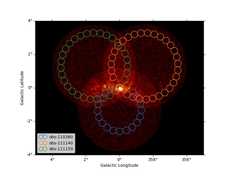
<WCSAxes: >
Model fit#
The next step is to fit a spectral model, using all data (i.e. a “global” fit, using all energies).
spectral_model = PowerLawSpectralModel(
    index=2, amplitude=1e-11 * u.Unit("cm-2 s-1 TeV-1"), reference=1 * u.TeV
)

model = SkyModel(spectral_model=spectral_model, name="source-gc")

datasets.models = model

fit = Fit()
result = fit.run(datasets=datasets)
print(result)
OptimizeResult

        backend    : minuit
        method     : migrad
        success    : True
        message    : Optimization terminated successfully.
        nfev       : 104
        total stat : 88.36

CovarianceResult

        backend    : minuit
        method     : hesse
        success    : True
        message    : Hesse terminated successfully.
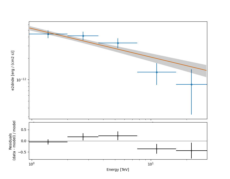
Spectral points#
Finally, let’s compute spectral points. The method used is to first choose an energy binning, and then to do a 1-dim likelihood fit / profile to compute the flux and flux error.
# Flux points are computed on stacked observation
stacked_dataset = datasets.stack_reduce(name="stacked")

print(stacked_dataset)

energy_edges = MapAxis.from_energy_bounds("1 TeV", "30 TeV", nbin=5).edges

stacked_dataset.models = model

fpe = FluxPointsEstimator(energy_edges=energy_edges, source="source-gc")
flux_points = fpe.run(datasets=[stacked_dataset])
flux_points.to_table(sed_type="dnde", formatted=True)
SpectrumDatasetOnOff
--------------------

  Name                            : stacked

  Total counts                    : 413
  Total background counts         : 85.43
  Total excess counts             : 327.57

  Predicted counts                : 98.34
  Predicted background counts     : 98.34
  Predicted excess counts         : nan

  Exposure min                    : 9.94e+07 m2 s
  Exposure max                    : 2.46e+10 m2 s

  Number of total bins            : 40
  Number of fit bins              : 30

  Fit statistic type              : wstat
  Fit statistic value (-2 log(L)) : 658.76

  Number of models                : 0
  Number of parameters            : 0
  Number of free parameters       : 0

  Total counts_off                : 2095
  Acceptance                      : 40
  Acceptance off                  : 990
Plot#
Let’s plot the spectral model and points. You could do it directly, but
for convenience we bundle the model and the flux points in a
FluxPointDataset:
flux_points_dataset = FluxPointsDataset(data=flux_points, models=model)
flux_points_dataset.plot_fit()
plt.show()
Exercises#
Re-run the analysis above, varying some analysis parameters, e.g.
Select a few other observations
Change the energy band for the map
Change the spectral model for the fit
Change the energy binning for the spectral points
Change the target. Make a sky image and spectrum for your favourite source.
If you don’t know any, the Crab nebula is the “hello world!” analysis of gamma-ray astronomy.
# print('hello world')
# SkyCoord.from_name('crab')
What next?#
This notebook showed an example of a first CTA analysis with Gammapy, using simulated 1DC data.
Let us know if you have any question or issues!
Total running time of the script: ( 0 minutes 23.150 seconds)