Note
Go to the end to download the full example code or to run this example in your browser via Binder
3D map simulation#
Simulate a 3D observation of a source with the CTA 1DC response and fit it with the assumed source model.
Prerequisites#
Knowledge of 3D extraction and datasets used in gammapy, see for example the High level interface tutorial.
Context#
To simulate a specific observation, it is not always necessary to simulate the full photon list. For many uses cases, simulating directly a reduced binned dataset is enough: the IRFs reduced in the correct geometry are combined with a source model to predict an actual number of counts per bin. The latter is then used to simulate a reduced dataset using Poisson probability distribution.
This can be done to check the feasibility of a measurement (performance / sensitivity study), to test whether fitted parameters really provide a good fit to the data etc.
Here we will see how to perform a 3D simulation of a CTA observation, assuming both the spectral and spatial morphology of an observed source.
Objective: simulate a 3D observation of a source with CTA using the CTA 1DC response and fit it with the assumed source model.
Proposed approach#
Here we can’t use the regular observation objects that are connected to
a DataStore. Instead we will create a fake
Observation that contain some pointing information and
the CTA 1DC IRFs (that are loaded with load_cta_irfs).
Then we will create a MapDataset geometry and
create it with the MapDatasetMaker.
Then we will be able to define a model consisting of a
PowerLawSpectralModel and a
GaussianSpatialModel. We will assign it to
the dataset and fake the count data.
Imports and versions#
import numpy as np
import astropy.units as u
from astropy.coordinates import SkyCoord
import matplotlib.pyplot as plt

# %matplotlib inline
from IPython.display import display
from gammapy.data import Observation, observatory_locations
from gammapy.datasets import MapDataset
from gammapy.irf import load_cta_irfs
from gammapy.makers import MapDatasetMaker, SafeMaskMaker
from gammapy.maps import MapAxis, WcsGeom
from gammapy.modeling import Fit
from gammapy.modeling.models import (
    FoVBackgroundModel,
    GaussianSpatialModel,
    Models,
    PowerLawSpectralModel,
    SkyModel,
)
Simulation#
We will simulate using the CTA-1DC IRFs shipped with gammapy
# Loading IRFs
irfs = load_cta_irfs(
    "$GAMMAPY_DATA/cta-1dc/caldb/data/cta/1dc/bcf/South_z20_50h/irf_file.fits"
)

# Define the observation parameters (typically the observation duration and the pointing position):
livetime = 2.0 * u.hr
pointing = SkyCoord(0, 0, unit="deg", frame="galactic")

# Define map geometry for binned simulation
energy_reco = MapAxis.from_edges(
    np.logspace(-1.0, 1.0, 10), unit="TeV", name="energy", interp="log"
)
geom = WcsGeom.create(
    skydir=(0, 0),
    binsz=0.02,
    width=(6, 6),
    frame="galactic",
    axes=[energy_reco],
)
# It is usually useful to have a separate binning for the true energy axis
energy_true = MapAxis.from_edges(
    np.logspace(-1.5, 1.5, 30), unit="TeV", name="energy_true", interp="log"
)

empty = MapDataset.create(geom, name="dataset-simu", energy_axis_true=energy_true)

# Define sky model to used simulate the data.
# Here we use a Gaussian spatial model and a Power Law spectral model.
spatial_model = GaussianSpatialModel(
    lon_0="0.2 deg", lat_0="0.1 deg", sigma="0.3 deg", frame="galactic"
)
spectral_model = PowerLawSpectralModel(
    index=3, amplitude="1e-11 cm-2 s-1 TeV-1", reference="1 TeV"
)
model_simu = SkyModel(
    spatial_model=spatial_model,
    spectral_model=spectral_model,
    name="model-simu",
)

bkg_model = FoVBackgroundModel(dataset_name="dataset-simu")

models = Models([model_simu, bkg_model])
print(models)
/home/runner/work/gammapy-docs/gammapy-docs/gammapy/.tox/build_docs/lib/python3.9/site-packages/astropy/units/core.py:2097: UnitsWarning: '1/s/MeV/sr' did not parse as fits unit: Numeric factor not supported by FITS If this is meant to be a custom unit, define it with 'u.def_unit'. To have it recognized inside a file reader or other code, enable it with 'u.add_enabled_units'. For details, see https://docs.astropy.org/en/latest/units/combining_and_defining.html
  warnings.warn(msg, UnitsWarning)
Models

Component 0: SkyModel

  Name                      : model-simu
  Datasets names            : None
  Spectral model type       : PowerLawSpectralModel
  Spatial  model type       : GaussianSpatialModel
  Temporal model type       :
  Parameters:
    index                         :      3.000   +/-    0.00
    amplitude                     :   1.00e-11   +/- 0.0e+00 1 / (cm2 s TeV)
    reference             (frozen):      1.000       TeV
    lon_0                         :      0.200   +/-    0.00 deg
    lat_0                         :      0.100   +/-    0.00 deg
    sigma                         :      0.300   +/-    0.00 deg
    e                     (frozen):      0.000
    phi                   (frozen):      0.000       deg

Component 1: FoVBackgroundModel

  Name                      : dataset-simu-bkg
  Datasets names            : ['dataset-simu']
  Spectral model type       : PowerLawNormSpectralModel
  Parameters:
    norm                          :      1.000   +/-    0.00
    tilt                  (frozen):      0.000
    reference             (frozen):      1.000       TeV
Now, comes the main part of dataset simulation. We create an in-memory
observation and an empty dataset. We then predict the number of counts
for the given model, and Poission fluctuate it using fake() to make
a simulated counts maps. Keep in mind that it is important to specify
the selection of the maps that you want to produce
# Create an in-memory observation
location = observatory_locations["cta_south"]
obs = Observation.create(
    pointing=pointing, livetime=livetime, irfs=irfs, location=location
)
print(obs)

# Make the MapDataset
maker = MapDatasetMaker(selection=["exposure", "background", "psf", "edisp"])

maker_safe_mask = SafeMaskMaker(methods=["offset-max"], offset_max=4.0 * u.deg)

dataset = maker.run(empty, obs)
dataset = maker_safe_mask.run(dataset, obs)
print(dataset)

# Add the model on the dataset and Poission fluctuate
dataset.models = models
dataset.fake()
# Do a print on the dataset - there is now a counts maps
print(dataset)
Observation

        obs id            : 0
        tstart            : 51544.00
        tstop             : 51544.08
        duration          : 7200.00 s
        pointing (icrs)   : 266.4 deg, -28.9 deg

        deadtime fraction : 0.0%

MapDataset
----------

  Name                            : dataset-simu

  Total counts                    : 0
  Total background counts         : 161250.95
  Total excess counts             : -161250.95

  Predicted counts                : 161250.95
  Predicted background counts     : 161250.95
  Predicted excess counts         : nan

  Exposure min                    : 4.08e+02 m2 s
  Exposure max                    : 3.58e+10 m2 s

  Number of total bins            : 810000
  Number of fit bins              : 804492

  Fit statistic type              : cash
  Fit statistic value (-2 log(L)) : nan

  Number of models                : 0
  Number of parameters            : 0
  Number of free parameters       : 0


MapDataset
----------

  Name                            : dataset-simu

  Total counts                    : 169814
  Total background counts         : 161250.95
  Total excess counts             : 8563.05

  Predicted counts                : 169871.61
  Predicted background counts     : 161250.95
  Predicted excess counts         : 8620.66

  Exposure min                    : 4.08e+02 m2 s
  Exposure max                    : 3.58e+10 m2 s

  Number of total bins            : 810000
  Number of fit bins              : 804492

  Fit statistic type              : cash
  Fit statistic value (-2 log(L)) : 563242.59

  Number of models                : 2
  Number of parameters            : 11
  Number of free parameters       : 6

  Component 0: SkyModel

    Name                      : model-simu
    Datasets names            : None
    Spectral model type       : PowerLawSpectralModel
    Spatial  model type       : GaussianSpatialModel
    Temporal model type       :
    Parameters:
      index                         :      3.000   +/-    0.00
      amplitude                     :   1.00e-11   +/- 0.0e+00 1 / (cm2 s TeV)
      reference             (frozen):      1.000       TeV
      lon_0                         :      0.200   +/-    0.00 deg
      lat_0                         :      0.100   +/-    0.00 deg
      sigma                         :      0.300   +/-    0.00 deg
      e                     (frozen):      0.000
      phi                   (frozen):      0.000       deg

  Component 1: FoVBackgroundModel

    Name                      : dataset-simu-bkg
    Datasets names            : ['dataset-simu']
    Spectral model type       : PowerLawNormSpectralModel
    Parameters:
      norm                          :      1.000   +/-    0.00
      tilt                  (frozen):      0.000
      reference             (frozen):      1.000       TeV
Now use this dataset as you would in all standard analysis. You can plot the maps, or proceed with your custom analysis. In the next section, we show the standard 3D fitting as in 3D detailed analysis tutorial.
# To plot, eg, counts:
plt.figure()
dataset.counts.smooth(0.05 * u.deg).plot_interactive(add_cbar=True, stretch="linear")
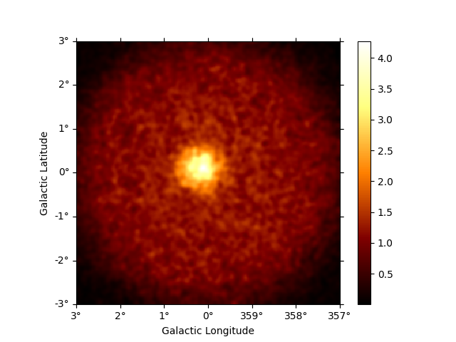
interactive(children=(SelectionSlider(continuous_update=False, description='Select energy:', layout=Layout(width='50%'), options=('100 GeV - 167 GeV', '167 GeV - 278 GeV', '278 GeV - 464 GeV', '464 GeV - 774 GeV', '774 GeV - 1.29 TeV', '1.29 TeV - 2.15 TeV', '2.15 TeV - 3.59 TeV', '3.59 TeV - 5.99 TeV', '5.99 TeV - 10.00 TeV'), style=SliderStyle(description_width='initial'), value='100 GeV - 167 GeV'), RadioButtons(description='Select stretch:', options=('linear', 'sqrt', 'log'), style=DescriptionStyle(description_width='initial'), value='linear'), Output()), _dom_classes=('widget-interact',))
Fit#
In this section, we do a usual 3D fit with the same model used to simulated the data and see the stability of the simulations. Often, it is useful to simulate many such datasets and look at the distribution of the reconstructed parameters.
models_fit = models.copy()

# We do not want to fit the background in this case, so we will freeze the parameters
models_fit["dataset-simu-bkg"].spectral_model.norm.frozen = True
models_fit["dataset-simu-bkg"].spectral_model.tilt.frozen = True

dataset.models = models_fit
print(dataset.models)
DatasetModels

Component 0: SkyModel

  Name                      : model-simu
  Datasets names            : None
  Spectral model type       : PowerLawSpectralModel
  Spatial  model type       : GaussianSpatialModel
  Temporal model type       :
  Parameters:
    index                         :      3.000   +/-    0.00
    amplitude                     :   1.00e-11   +/- 0.0e+00 1 / (cm2 s TeV)
    reference             (frozen):      1.000       TeV
    lon_0                         :      0.200   +/-    0.00 deg
    lat_0                         :      0.100   +/-    0.00 deg
    sigma                         :      0.300   +/-    0.00 deg
    e                     (frozen):      0.000
    phi                   (frozen):      0.000       deg

Component 1: FoVBackgroundModel

  Name                      : dataset-simu-bkg
  Datasets names            : ['dataset-simu']
  Spectral model type       : PowerLawNormSpectralModel
  Parameters:
    norm                  (frozen):      1.000
    tilt                  (frozen):      0.000
    reference             (frozen):      1.000       TeV
fit = Fit(optimize_opts={"print_level": 1})
result = fit.run(datasets=[dataset])
plt.figure()
dataset.plot_residuals_spatial(method="diff/sqrt(model)", vmin=-0.5, vmax=0.5)
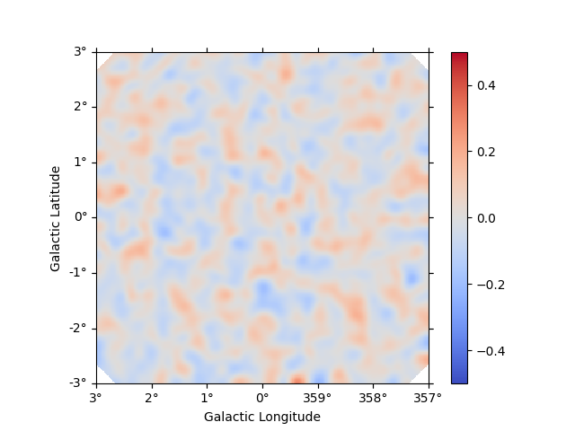
<WCSAxes: >
Compare the injected and fitted models:
print(
    "True model: \n",
    model_simu,
    "\n\n Fitted model: \n",
    models_fit["model-simu"],
)
True model:
 SkyModel

  Name                      : model-simu
  Datasets names            : None
  Spectral model type       : PowerLawSpectralModel
  Spatial  model type       : GaussianSpatialModel
  Temporal model type       :
  Parameters:
    index                         :      3.000   +/-    0.00
    amplitude                     :   1.00e-11   +/- 0.0e+00 1 / (cm2 s TeV)
    reference             (frozen):      1.000       TeV
    lon_0                         :      0.200   +/-    0.00 deg
    lat_0                         :      0.100   +/-    0.00 deg
    sigma                         :      0.300   +/-    0.00 deg
    e                     (frozen):      0.000
    phi                   (frozen):      0.000       deg


 Fitted model:
 SkyModel

  Name                      : model-simu
  Datasets names            : None
  Spectral model type       : PowerLawSpectralModel
  Spatial  model type       : GaussianSpatialModel
  Temporal model type       :
  Parameters:
    index                         :      3.023   +/-    0.02
    amplitude                     :   9.70e-12   +/- 3.3e-13 1 / (cm2 s TeV)
    reference             (frozen):      1.000       TeV
    lon_0                         :      0.183   +/-    0.01 deg
    lat_0                         :      0.099   +/-    0.01 deg
    sigma                         :      0.299   +/-    0.00 deg
    e                     (frozen):      0.000
    phi                   (frozen):      0.000       deg
Get the errors on the fitted parameters from the parameter table
display(result.parameters.to_table())

plt.show()
  type      name     value         unit      ...    max    frozen is_norm link
-------- --------- ---------- -------------- ... --------- ------ ------- ----
spectral     index 3.0227e+00                ...       nan  False   False
spectral amplitude 9.7023e-12 cm-2 s-1 TeV-1 ...       nan  False    True
spectral reference 1.0000e+00            TeV ...       nan   True   False
 spatial     lon_0 1.8262e-01            deg ...       nan  False   False
 spatial     lat_0 9.8898e-02            deg ... 9.000e+01  False   False
 spatial     sigma 2.9890e-01            deg ...       nan  False   False
 spatial         e 0.0000e+00                ... 1.000e+00   True   False
 spatial       phi 0.0000e+00            deg ...       nan   True   False
spectral      norm 1.0000e+00                ...       nan   True    True
spectral      tilt 0.0000e+00                ...       nan   True   False
spectral reference 1.0000e+00            TeV ...       nan   True   False
Total running time of the script: ( 0 minutes 19.992 seconds)