Note
Go to the end to download the full example code or to run this example in your browser via Binder
Event sampling#
Learn to sampling events from a given sky model and IRFs.
Prerequisites#
To understand how to generate a model and a MapDataset and how to fit
the data, please refer to the SkyModel and
3D map simulation tutorial.
Context#
This tutorial describes how to sample events from an observation of a one (or more) gamma-ray source(s). The main aim of the tutorial will be to set the minimal configuration needed to deal with the Gammapy event-sampler and how to obtain an output photon event list.
The core of the event sampling lies into the Gammapy
MapDatasetEventSampler class, which is based on
the inverse cumulative distribution function (Inverse
CDF).
The MapDatasetEventSampler takes in input a
Dataset object containing the spectral, spatial
and temporal properties of the source(s) of interest.
The MapDatasetEventSampler class evaluates the map
of predicted counts (npred) per bin of the given Sky model, and the
npred map is then used to sample the events. In particular, the
output of the event-sampler will be a set of events having information
about their true coordinates, true energies and times of arrival.
To these events, IRF corrections (i.e. PSF and energy dispersion) can also further applied in order to obtain reconstructed coordinates and energies of the sampled events.
At the end of this process, you will obtain an event-list in FITS format.
Objective#
Describe the process of sampling events from a given Sky model and obtain an output event-list.
Proposed approach#
In this section, we will show how to define an observation and create a Dataset object. These are both necessary for the event sampling. Then, we will define the Sky model from which we sample events.
In this tutorial, we propose examples for sampling events of:
We will work with the following functions and classes:
Setup#
As usual, let’s start with some general imports…
from pathlib import Path
import numpy as np
import astropy.units as u
from astropy.coordinates import Angle, SkyCoord
from astropy.io import fits
from astropy.time import Time
from regions import CircleSkyRegion
import matplotlib.pyplot as plt

# %matplotlib inline
from IPython.display import display
from gammapy.data import DataStore, Observation, observatory_locations
from gammapy.datasets import MapDataset, MapDatasetEventSampler
from gammapy.irf import load_cta_irfs
from gammapy.makers import MapDatasetMaker
from gammapy.maps import Map, MapAxis, WcsGeom
from gammapy.modeling import Fit
from gammapy.modeling.models import (
    ExpDecayTemporalModel,
    FoVBackgroundModel,
    Models,
    PointSpatialModel,
    PowerLawNormSpectralModel,
    PowerLawSpectralModel,
    SkyModel,
    TemplateSpatialModel,
)
Check setup#
from gammapy.utils.check import check_tutorials_setup

check_tutorials_setup()
System:

        python_executable      : /home/runner/work/gammapy-docs/gammapy-docs/gammapy/.tox/build_docs/bin/python
        python_version         : 3.9.16
        machine                : x86_64
        system                 : Linux


Gammapy package:

        version                : 1.0.1
        path                   : /home/runner/work/gammapy-docs/gammapy-docs/gammapy/.tox/build_docs/lib/python3.9/site-packages/gammapy


Other packages:

        numpy                  : 1.24.2
        scipy                  : 1.10.1
        astropy                : 5.2.1
        regions                : 0.7
        click                  : 8.1.3
        yaml                   : 6.0
        IPython                : 8.11.0
        jupyterlab             : not installed
        matplotlib             : 3.7.1
        pandas                 : not installed
        healpy                 : 1.16.2
        iminuit                : 2.21.0
        sherpa                 : 4.15.0
        naima                  : 0.10.0
        emcee                  : 3.1.4
        corner                 : 2.2.1


Gammapy environment variables:

        GAMMAPY_DATA           : /home/runner/work/gammapy-docs/gammapy-docs/gammapy-datasets/1.0.1
Define an Observation#
You can firstly create a Observations object that
contains the pointing position, the GTIs and the IRF you want to
consider.
Hereafter, we chose the IRF of the South configuration used for the CTA DC1 and we set the pointing position of the simulated field at the Galactic Center. We also fix the exposure time to 1 hr.
Let’s start with some initial settings:
Now you can create the observation:
irfs = load_cta_irfs(path / irf_filename)
location = observatory_locations["cta_south"]

observation = Observation.create(
    obs_id=1001,
    pointing=pointing,
    livetime=livetime,
    irfs=irfs,
    location=location,
)
Define the MapDataset#
Let’s generate the Dataset object (for more info
on Dataset objects, please checkout
Datasets - Reduced data, IRFs, models tutorial):
we define the energy axes (true and reconstruncted), the migration axis
and the geometry of the observation.
This is a crucial point for the correct configuration of the event sampler. Indeed the spatial and energetic binning should be treaten carefully and… the finer the better. For this reason, we suggest to define the energy axes (true and reconstructed) by setting a minimum binning of least 10-20 bins per decade for all the sources of interest. The spatial binning may instead be different from source to source and, at first order, it should be adopted a binning significantly smaller than the expected source size.
For the examples that will be shown hereafter, we set the geometry of the dataset to a field of view of 2degx2deg and we bin the spatial map with pixels of 0.02 deg.
energy_axis = MapAxis.from_energy_bounds("0.1 TeV", "100 TeV", nbin=10, per_decade=True)
energy_axis_true = MapAxis.from_energy_bounds(
    "0.03 TeV", "300 TeV", nbin=20, per_decade=True, name="energy_true"
)
migra_axis = MapAxis.from_bounds(0.5, 2, nbin=150, node_type="edges", name="migra")

geom = WcsGeom.create(
    skydir=pointing,
    width=(2, 2),
    binsz=0.02,
    frame="galactic",
    axes=[energy_axis],
)
In the following, the dataset is created by selecting the effective
area, background model, the PSF and the Edisp from the IRF. The dataset
thus produced can be saved into a FITS file just using the write()
function. We put it into the evt_sampling sub-folder:
empty = MapDataset.create(
    geom,
    energy_axis_true=energy_axis_true,
    migra_axis=migra_axis,
    name="my-dataset",
)
maker = MapDatasetMaker(selection=["exposure", "background", "psf", "edisp"])
dataset = maker.run(empty, observation)

Path("event_sampling").mkdir(exist_ok=True)
dataset.write("./event_sampling/dataset.fits", overwrite=True)
Define the Sky model: a point-like source#
Now let’s define a sky model for a point-like source centered 0.5 deg far from the Galactic Center and with a power-law spectrum. We then save the model into a yaml file.
spectral_model_pwl = PowerLawSpectralModel(
    index=2, amplitude="1e-12 TeV-1 cm-2 s-1", reference="1 TeV"
)
spatial_model_point = PointSpatialModel(
    lon_0="0 deg", lat_0="0.5 deg", frame="galactic"
)

sky_model_pntpwl = SkyModel(
    spectral_model=spectral_model_pwl,
    spatial_model=spatial_model_point,
    name="point-pwl",
)

bkg_model = FoVBackgroundModel(dataset_name="my-dataset")

models = Models([sky_model_pntpwl, bkg_model])

file_model = "./event_sampling/point-pwl.yaml"
models.write(file_model, overwrite=True)
Sampling the source and background events#
Now, we can finally add the SkyModel we
want to event-sample to the Dataset container:
dataset.models = models
print(dataset.models)
DatasetModels

Component 0: SkyModel

  Name                      : point-pwl
  Datasets names            : None
  Spectral model type       : PowerLawSpectralModel
  Spatial  model type       : PointSpatialModel
  Temporal model type       :
  Parameters:
    index                         :      2.000   +/-    0.00
    amplitude                     :   1.00e-12   +/- 0.0e+00 1 / (cm2 s TeV)
    reference             (frozen):      1.000       TeV
    lon_0                         :      0.000   +/-    0.00 deg
    lat_0                         :      0.500   +/-    0.00 deg

Component 1: FoVBackgroundModel

  Name                      : my-dataset-bkg
  Datasets names            : ['my-dataset']
  Spectral model type       : PowerLawNormSpectralModel
  Parameters:
    norm                          :      1.000   +/-    0.00
    tilt                  (frozen):      0.000
    reference             (frozen):      1.000       TeV
The next step shows how to sample the events with the
MapDatasetEventSampler class. The class requests a
random number seed generator (that we set with random_state=0), the
Dataset and the Observations
object. From the latter, the
MapDatasetEventSampler class takes all the meta
data information.
sampler = MapDatasetEventSampler(random_state=0)
events = sampler.run(dataset, observation)
The output of the event-sampler is an event list with coordinates,
energies (true and reconstructed) and time of arrivals of the source and
background events. events is a EventList object
(for details see e.g. CTA with Gammapy tutorial.).
Source and background events are flagged by the MC_ID identifier (where
0 is the default identifier for the background).
print(f"Source events: {(events.table['MC_ID'] == 1).sum()}")
print(f"Background events: {(events.table['MC_ID'] == 0).sum()}")
Source events: 138
Background events: 15319
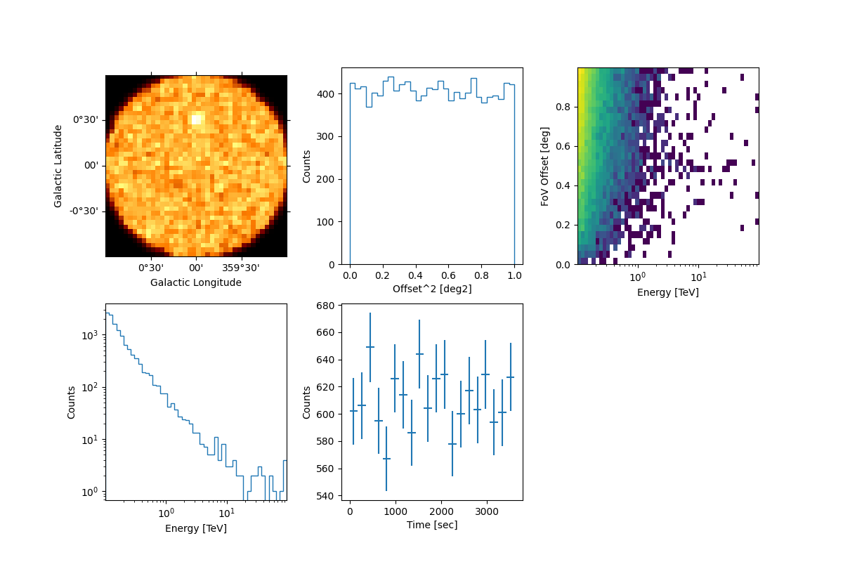
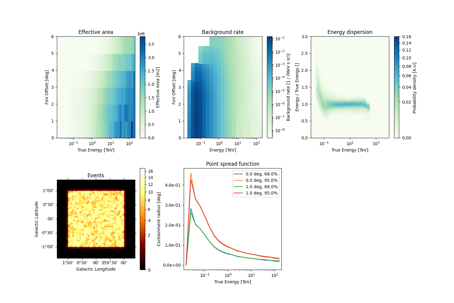
We can inspect the properties of the simulated events as follows:
events.select_offset([0, 1] * u.deg).peek()
By default, the MapDatasetEventSampler fills the
metadata keyword OBJECT in the event list using the first model of
the SkyModel object. You can change it with the following commands:
events.table.meta["OBJECT"] = dataset.models[0].name
Let’s write the event list and its GTI extension to a FITS file. We make
use of fits library in astropy:
primary_hdu = fits.PrimaryHDU()
hdu_evt = fits.BinTableHDU(events.table)
hdu_gti = fits.BinTableHDU(dataset.gti.table, name="GTI")
hdu_all = fits.HDUList([primary_hdu, hdu_evt, hdu_gti])
hdu_all.writeto("./event_sampling/events_0001.fits", overwrite=True)
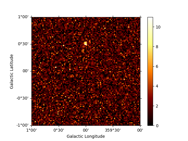
Generate a skymap#
A skymap of the simulated events can be obtained with:
counts = Map.from_geom(geom)
counts.fill_events(events)
plt.figure()
counts.sum_over_axes().plot(add_cbar=True)
<WCSAxes: >
Fit the simulated data#
- We can now check the sake of the event sampling by fitting the data.
We make use of the same
Models adopted for the simulation. Hence,
we firstly read the Dataset and the model file,
and we fill the Dataset with the sampled events.
We set the counts map to the dataset:
models_fit = Models.read("./event_sampling/point-pwl.yaml")

dataset.counts = counts
dataset.models = models_fit
Let’s fit the data and look at the results:
OptimizeResult

        backend    : minuit
        method     : migrad
        success    : True
        message    : Optimization terminated successfully.
        nfev       : 102
        total stat : 76403.35

CovarianceResult

        backend    : minuit
        method     : hesse
        success    : True
        message    : Hesse terminated successfully.
The results looks great!
Time variable source using a lightcurve#
The event sampler can also handle temporal variability of the simulated sources. In this example, we show how to sample a source characterized by an exponential decay, with decay time of 2800 seconds, during the observation.
First of all, let’s create a lightcurve:
t0 = 2800 * u.s
t_ref = Time("2000-01-01T00:01:04.184")

times = t_ref + livetime * np.linspace(0, 1, 100)
expdecay_model = ExpDecayTemporalModel(t_ref=t_ref.mjd * u.d, t0=t0)
where we defined the time axis starting from the reference time
t_ref up to the requested exposure (livetime). The bin size of
the time-axis is quite arbitrary but, as above for spatial and energy
binnings, the finer the better.
Then, we can create the sky model. Just for the sake of the example, let’s boost the flux of the simulated source of an order of magnitude:
spectral_model_pwl.amplitude.value = 2e-11

sky_model_pntpwl = SkyModel(
    spectral_model=spectral_model_pwl,
    spatial_model=spatial_model_point,
    temporal_model=expdecay_model,
    name="point-pwl",
)

bkg_model = FoVBackgroundModel(dataset_name="my-dataset")

models = Models([sky_model_pntpwl, bkg_model])

file_model = "./event_sampling/point-pwl_decay.yaml"
models.write(file_model, overwrite=True)
For simplicity, we use the same dataset defined for the previous example:
dataset.models = models
print(dataset.models)
DatasetModels

Component 0: SkyModel

  Name                      : point-pwl
  Datasets names            : None
  Spectral model type       : PowerLawSpectralModel
  Spatial  model type       : PointSpatialModel
  Temporal model type       : ExpDecayTemporalModel
  Parameters:
    index                         :      2.000   +/-    0.00
    amplitude                     :   2.00e-11   +/- 0.0e+00 1 / (cm2 s TeV)
    reference             (frozen):      1.000       TeV
    lon_0                         :      0.000   +/-    0.00 deg
    lat_0                         :      0.500   +/-    0.00 deg
    t0                            :   2800.000   +/-    0.00 s
    t_ref                 (frozen):  51544.001       d

Component 1: FoVBackgroundModel

  Name                      : my-dataset-bkg
  Datasets names            : ['my-dataset']
  Spectral model type       : PowerLawNormSpectralModel
  Parameters:
    norm                          :      1.000   +/-    0.00
    tilt                  (frozen):      0.000
    reference             (frozen):      1.000       TeV
And now, let’s simulate the variable source:
sampler = MapDatasetEventSampler(random_state=0)
events = sampler.run(dataset, observation)

print(f"Source events: {(events.table['MC_ID'] == 1).sum()}")
print(f"Background events: {(events.table['MC_ID'] == 0).sum()}")
Source events: 1523
Background events: 15246
We can now inspect the properties of the simulated source. To do that,
we adopt the select_region function that extracts only the events
into a given SkyRegion of a EventList object:
src_position = SkyCoord(0.0, 0.5, frame="galactic", unit="deg")

on_region_radius = Angle("0.15 deg")
on_region = CircleSkyRegion(center=src_position, radius=on_region_radius)

src_events = events.select_region(on_region)
Then we can have a quick look to the data with the peek function:
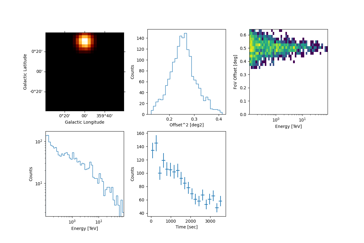
In the right figure of the bottom panel, it is shown the source lightcurve that follows a decay trend as expected.
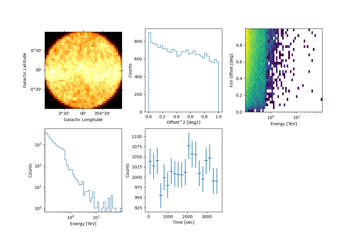
Extended source using a template#
The event sampler can also work with a template model. Here we use the interstellar emission model map of the Fermi 3FHL, which can be found in the GAMMAPY data repository.
We proceed following the same steps showed above and we finally have a look at the event’s properties:
template_model = TemplateSpatialModel.read(
    "$GAMMAPY_DATA/fermi-3fhl-gc/gll_iem_v06_gc.fits.gz", normalize=False
)
# we make the model brighter artificially so that it becomes visible over the background
diffuse = SkyModel(
    spectral_model=PowerLawNormSpectralModel(norm=5),
    spatial_model=template_model,
    name="template-model",
)

bkg_model = FoVBackgroundModel(dataset_name="my-dataset")

models_diffuse = Models([diffuse, bkg_model])

file_model = "./event_sampling/diffuse.yaml"
models_diffuse.write(file_model, overwrite=True)

dataset.models = models_diffuse
print(dataset.models)
DatasetModels

Component 0: SkyModel

  Name                      : template-model
  Datasets names            : None
  Spectral model type       : PowerLawNormSpectralModel
  Spatial  model type       : TemplateSpatialModel
  Temporal model type       :
  Parameters:
    norm                          :      5.000   +/-    0.00
    tilt                  (frozen):      0.000
    reference             (frozen):      1.000       TeV

Component 1: FoVBackgroundModel

  Name                      : my-dataset-bkg
  Datasets names            : ['my-dataset']
  Spectral model type       : PowerLawNormSpectralModel
  Parameters:
    norm                          :      1.000   +/-    0.00
    tilt                  (frozen):      0.000
    reference             (frozen):      1.000       TeV
sampler = MapDatasetEventSampler(random_state=0)
events = sampler.run(dataset, observation)

events.select_offset([0, 1] * u.deg).peek()
Simulate multiple event lists#
In some user case, you may want to sample events from a number of observations. In this section, we show how to simulate a set of event lists. For simplicity we consider only one point-like source, observed three times for 1 hr and assuming the same pointing position.
Let’s firstly define the time start and the livetime of each observation:
n_obs = len(tstarts)
irf_paths = [path / irf_filename] * n_obs
events_paths = []

for idx, tstart in enumerate(tstarts):
    irfs = load_cta_irfs(irf_paths[idx])
    observation = Observation.create(
        obs_id=idx,
        pointing=pointing,
        tstart=tstart,
        livetime=livetimes[idx],
        irfs=irfs,
        location=location,
    )

    dataset = maker.run(empty, observation)
    dataset.models = models
    sampler = MapDatasetEventSampler(random_state=idx)
    events = sampler.run(dataset, observation)

    path = Path(f"./event_sampling/events_{idx:04d}.fits")
    events_paths.append(path)
    events.table.write(path, overwrite=True)
/home/runner/work/gammapy-docs/gammapy-docs/gammapy/.tox/build_docs/lib/python3.9/site-packages/gammapy/utils/random/inverse_cdf.py:35: RuntimeWarning: invalid value encountered in divide
  pdf = pdf.ravel() / pdf.sum()
/home/runner/work/gammapy-docs/gammapy-docs/gammapy/.tox/build_docs/lib/python3.9/site-packages/astropy/units/quantity.py:673: RuntimeWarning: invalid value encountered in divide
  result = super().__array_ufunc__(function, method, *arrays, **kwargs)
You can now load the event list and the corresponding IRFs with
DataStore.from_events_files :
path = Path("./event_sampling/")
events_paths = list(path.rglob("events*.fits"))
data_store = DataStore.from_events_files(events_paths, irf_paths)
display(data_store.obs_table)
OBS_ID ...
       ...
------ ...
     0 ...
     1 ...
     2 ...
Then you can create the obervations from the data store and make your own analysis following the instructions in the Low level API tutorial.
observations = data_store.get_observations()
observations[0].peek()

plt.show()
Exercises#
Try to sample events for an extended source (e.g. a radial gaussian morphology);
Change the spatial model and the spectrum of the simulated Sky model;
Include a temporal model in the simulation
Total running time of the script: ( 1 minutes 2.390 seconds)