H.E.S.S. with Gammapy

Explore H.E.S.S. event lists and IRFs.

H.E.S.S. is an array of gamma-ray telescopes located in Namibia. Gammapy is regularly used and fully supports H.E.S.S. high level data analysis, after export to the current open data level 3 format.

The H.E.S.S. data is private, and H.E.S.S. analysis is mostly documented and discussed at https://hess-confluence.desy.de/ and in H.E.S.S.-internal communication channels. However, in 2018, a small sub-set of archival H.E.S.S. data was publicly released, called the H.E.S.S. DL3 DR1, the data level 3, data release number 1. This dataset is 50 MB in size and is used in many Gammapy analysis tutorials, and can be downloaded via gammapy download.

This notebook is a quick introduction to this specific DR1 release. It briefly describes H.E.S.S. data and instrument responses and show a simple exploration of the data with the creation of theta-squared plot.

H.E.S.S. members can find details on the DL3 FITS production on this Confluence page and access more detailed tutorials in this repository

DL3 DR1

This is how to access data and IRFs from the H.E.S.S. data level 3, data release 1.

import astropy.units as u
from astropy.coordinates import SkyCoord
import matplotlib.pyplot as plt
from IPython.display import display
from gammapy.data import DataStore
from gammapy.makers import MapDatasetMaker
from gammapy.makers.utils import make_theta_squared_table
from gammapy.maps import Map, MapAxis, WcsGeom

Check setup

from gammapy.utils.check import check_tutorials_setup
from gammapy.visualization import plot_theta_squared_table

check_tutorials_setup()

System:

        python_executable      : /home/runner/work/gammapy-docs/gammapy-docs/gammapy/.tox/build_docs/bin/python
        python_version         : 3.9.16
        machine                : x86_64
        system                 : Linux


Gammapy package:

        version                : 1.0.1
        path                   : /home/runner/work/gammapy-docs/gammapy-docs/gammapy/.tox/build_docs/lib/python3.9/site-packages/gammapy


Other packages:

        numpy                  : 1.24.2
        scipy                  : 1.10.1
        astropy                : 5.2.1
        regions                : 0.7
        click                  : 8.1.3
        yaml                   : 6.0
        IPython                : 8.11.0
        jupyterlab             : not installed
        matplotlib             : 3.7.1
        pandas                 : not installed
        healpy                 : 1.16.2
        iminuit                : 2.21.0
        sherpa                 : 4.15.0
        naima                  : 0.10.0
        emcee                  : 3.1.4
        corner                 : 2.2.1


Gammapy environment variables:

        GAMMAPY_DATA           : /home/runner/work/gammapy-docs/gammapy-docs/gammapy-datasets/1.0.1

A useful way to organize the relevant files are the index tables. The observation index table contains information on each particular run, such as the pointing, or the run ID. The HDU index table has a row per relevant file (i.e., events, effective area, psf…) and contains the path to said file. Together they can be loaded into a Datastore by indicating the directory in which they can be found, in this case “$GAMMAPY_DATA/hess-dl3-dr1”:

Create and get info on the data store

data_store = DataStore.from_dir("$GAMMAPY_DATA/hess-dl3-dr1")

data_store.info()

Data store:
HDU index table:
BASE_DIR: /home/runner/work/gammapy-docs/gammapy-docs/gammapy-datasets/1.0.1/hess-dl3-dr1
Rows: 630
OBS_ID: 20136 -- 47829
HDU_TYPE: ['aeff', 'bkg', 'edisp', 'events', 'gti', 'psf']
HDU_CLASS: ['aeff_2d', 'bkg_3d', 'edisp_2d', 'events', 'gti', 'psf_table']


Observation table:
Observatory name: 'N/A'
Number of observations: 105

Preview an excerpt from the observtaion table

display(data_store.obs_table[:2][["OBS_ID", "DATE-OBS", "RA_PNT", "DEC_PNT", "OBJECT"]])

OBS_ID  DATE-OBS   RA_PNT   DEC_PNT    OBJECT
                    deg       deg
------ ---------- -------- ---------- --------
 20136 2004-03-26 228.6125 -58.771667 MSH15-52
 20137 2004-03-26 228.6125 -59.771667 MSH15-52

Get a single obervation

obs = data_store.obs(23523)

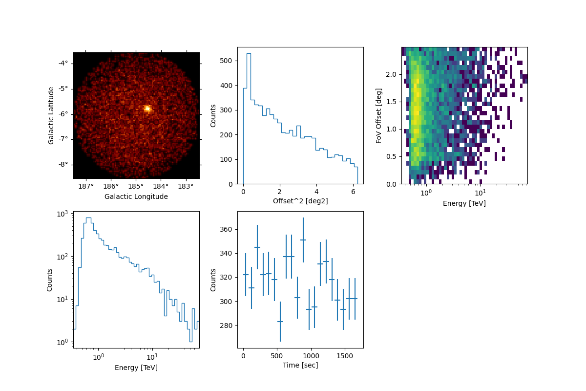
Select and peek events

obs.events.select_offset([0, 2.5] * u.deg).peek()

Peek the effective area

obs.aeff.peek()

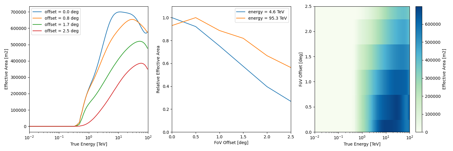
/home/runner/work/gammapy-docs/gammapy-docs/gammapy/.tox/build_docs/lib/python3.9/site-packages/astropy/units/quantity.py:673: RuntimeWarning: invalid value encountered in divide
  result = super().__array_ufunc__(function, method, *arrays, **kwargs)

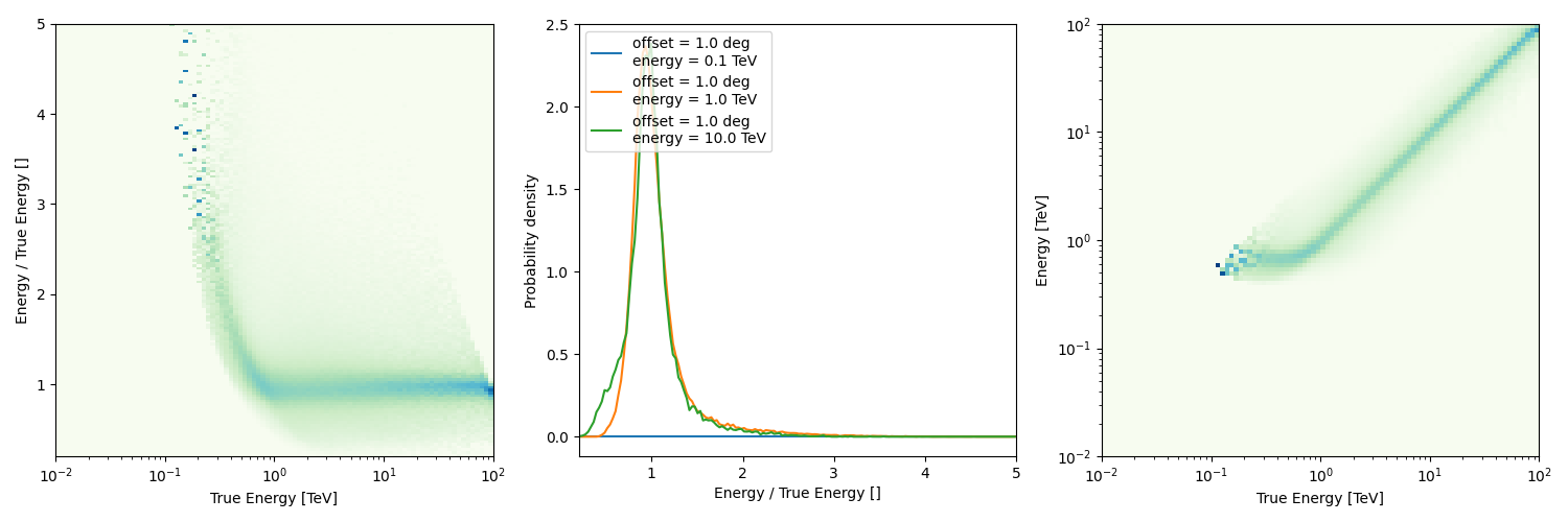
Peek the energy dispersion

obs.edisp.peek()

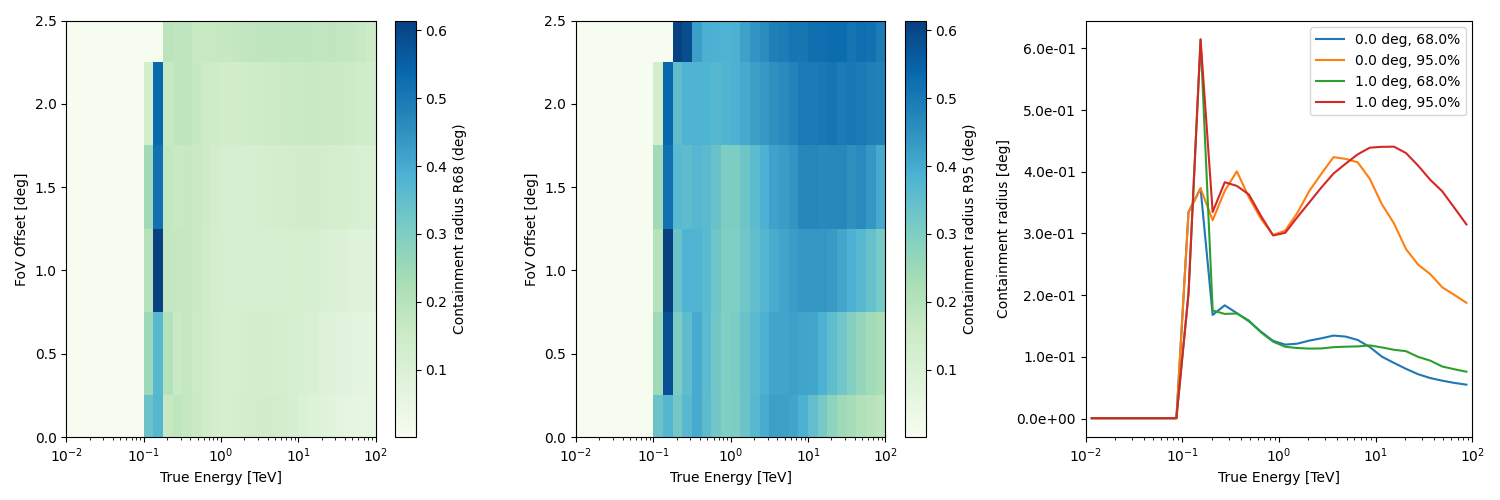
Peek the psf

obs.psf.peek()

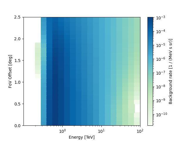
Peek the background rate

plt.figure()
obs.bkg.to_2d().plot()

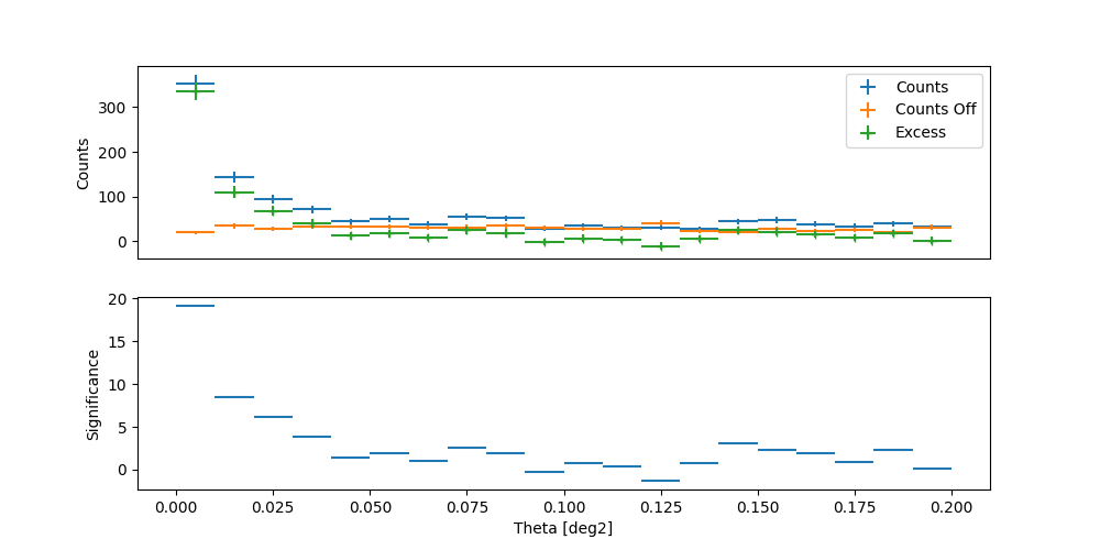
Theta squared event distribution

As a quick look plot it can be helpful to plot the quadratic offset (theta squared) distribution of the events.

position = SkyCoord(ra=83.63, dec=22.01, unit="deg", frame="icrs")
theta2_axis = MapAxis.from_bounds(0, 0.2, nbin=20, interp="lin", unit="deg2")

observations = data_store.get_observations([23523, 23526])
theta2_table = make_theta_squared_table(
    observations=observations,
    position=position,
    theta_squared_axis=theta2_axis,
)

plt.figure(figsize=(10, 5))
plot_theta_squared_table(theta2_table)

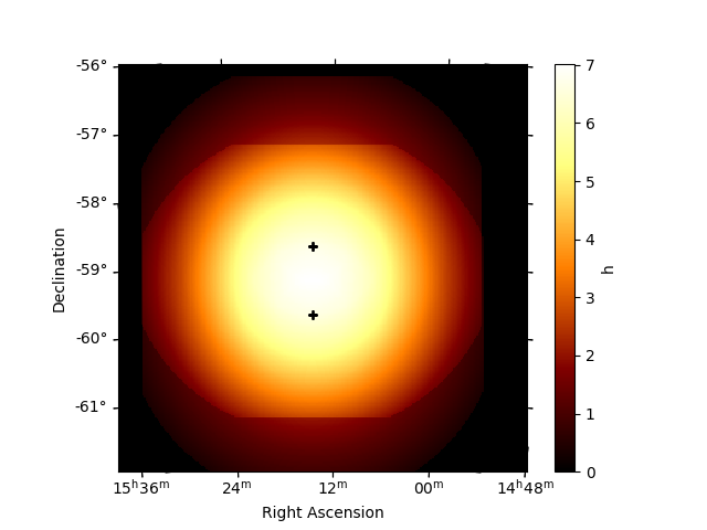
On-axis equivalent livetime

Since the acceptance of the H.E.S.S. camera varies within the field of view, what is often interesting is not the simply the total number of hours a source was observed, but the on-axis equivalent number of hours. We calculated the same for the MSH 1552 runs here.

# Get the observations
obs_id = data_store.obs_table["OBS_ID"][data_store.obs_table["OBJECT"] == "MSH 15-5-02"]
observations = data_store.get_observations(obs_id)
print("No. of observations: ", len(observations))

# Define an energy range
energy_min = 100 * u.GeV
energy_max = 10.0 * u.TeV

# define a offset cut
offset_max = 2.5 * u.deg

# define the geom
source_pos = SkyCoord(228.32, -59.08, unit="deg")
energy_axis_true = MapAxis.from_energy_bounds(
    energy_min, energy_max, nbin=1, name="energy_true"
)
geom = WcsGeom.create(
    skydir=source_pos,
    binsz=0.02,
    width=(6, 6),
    frame="icrs",
    proj="CAR",
    axes=[energy_axis_true],
)

# compute
livetime = Map.from_geom(geom, unit=u.hr)
for obs in observations:
    geom_obs = geom.cutout(position=obs.pointing_radec, width=2.0 * offset_max)
    exposure = MapDatasetMaker.make_exposure(geom=geom_obs, observation=obs)
    on_axis = obs.aeff.evaluate(
        offset=0.0 * u.deg, energy_true=geom.axes["energy_true"].center
    )
    on_axis = on_axis.reshape((on_axis.shape[0], 1, 1))
    lv_obs = exposure / on_axis
    livetime.stack(lv_obs)

# Plot
plt.figure()
ax = livetime.plot(add_cbar=True)

# Add the pointing position on top
for obs in observations:
    ax.plot(
        obs.pointing_radec.to_pixel(wcs=ax.wcs)[0],
        obs.pointing_radec.to_pixel(wcs=ax.wcs)[1],
        "+",
        color="black",
    )

plt.show()

No. of observations:  17

Exercises

• Find the OBS_ID for the runs of the Crab nebula

• Compute the expected number of background events in the whole RoI for OBS_ID=23523 in the 1 TeV to 3 TeV energy band, from the background IRF.

Next steps

Now you know how to access and work with H.E.S.S. data. All other tutorials and documentation apply to H.E.S.S. and CTA or any other IACT that provides DL3 data and IRFs in the standard format.