This is a fixed-text formatted version of a Jupyter notebook
- Try online

- You can contribute with your own notebooks in this GitHub repository.
- Source files: hess.ipynb | hess.py
Analysis of H.E.S.S. DL3 data with Gammapy
In September 2018 the H.E.S.S. collaboration released a small subset of archival data in FITS format. This tutorial explains how to analyse this data with Gammapy. We will analyse four observation runs of the Crab nebula, which are part of the H.E.S.S. first public test data release. The data was release without corresponding background models. In background_model.ipynb we show how to make a simple background model, which is also used in this tutorial. The background model is not perfect; it assumes radial symmetry and is in general derived from only a few observations, but still good enough for a reliable analysis > 1TeV.
Note: The high level Analysis class is a new feature added in Gammapy v0.14. In the curret state it supports the standard analysis cases of a joint or stacked 3D and 1D analysis. It provides only limited access to analaysis parameters via the config file. It is expected that the format of the YAML config will be extended and change in future Gammapy versions.
We will first show how to configure and run a stacked 3D analysis and then address the classical spectral analysis using reflected regions later. The structure of the tutorial follows a typical analysis:
- Analysis configuration
- Observation slection
- Data reduction
- Model fitting
- Estimating flux points
Finally we will compare the results against a reference model.
Setup
[1]:
%matplotlib inline
import matplotlib.pyplot as plt
import numpy as np
[2]:
import yaml
from pathlib import Path
from regions import CircleSkyRegion
from astropy import units as u
from astropy.coordinates import SkyCoord
from gammapy.scripts import Analysis, AnalysisConfig
from gammapy.modeling.models import create_crab_spectral_model
Analysis configuration
For configuration of the analysis we use the YAML data format. YAML is a machine readable serialisation format, that is also friendly for humans to read. In this tutorial we will write the configuration file just using Python strings, but of course the file can be created and modified with any text editor of your choice.
Here is what the configuration for our analysis looks like:
[3]:
config_str = """
general:
    logging:
        level: INFO
    outdir: .

observations:
    datastore: $GAMMAPY_DATA/hess-dl3-dr1/hess-dl3-dr3-with-background.fits.gz
    filters:
        - filter_type: par_value
          value_param: Crab
          variable: TARGET_NAME

datasets:
    dataset-type: MapDataset
    stack-datasets: true
    offset-max: 2.5 deg
    geom:
        skydir: [83.633, 22.014]
        width: [5, 5]
        binsz: 0.02
        coordsys: CEL
        proj: TAN
        axes:
          - name: energy
            hi_bnd: 10
            lo_bnd: 1
            nbin: 5
            interp: log
            node_type: edges
            unit: TeV

fit:
    fit_range:
        max: 30 TeV
        min: 1 TeV

flux-points:
    fp_binning:
        lo_bnd: 1
        hi_bnd: 10
        interp: log
        nbin: 3
        unit: TeV
"""
We first create an AnalysiConfig object from it:
[4]:
config = AnalysisConfig(config_str)
Observation selection
Now we create the high level Analysis object from the config object:
[5]:
analysis = Analysis(config)
INFO:gammapy.scripts.analysis:Setting logging config: {'level': 'INFO'}
And directly select and load the observatiosn from disk using .get_observations():
[6]:
analysis.get_observations()
INFO:gammapy.scripts.analysis:Fetching observations.
INFO:gammapy.scripts.analysis:Info for OBS_ID = 23592
- Start time: 53347.91
- Pointing pos: RA 82.01 deg / Dec 22.01 deg
- Observation duration: 1686.0 s
- Dead-time fraction: 6.212 %

INFO:gammapy.scripts.analysis:Info for OBS_ID = 23523
- Start time: 53343.92
- Pointing pos: RA 83.63 deg / Dec 21.51 deg
- Observation duration: 1687.0 s
- Dead-time fraction: 6.240 %

INFO:gammapy.scripts.analysis:Info for OBS_ID = 23526
- Start time: 53343.95
- Pointing pos: RA 83.63 deg / Dec 22.51 deg
- Observation duration: 1683.0 s
- Dead-time fraction: 6.555 %

INFO:gammapy.scripts.analysis:Info for OBS_ID = 23559
- Start time: 53345.96
- Pointing pos: RA 85.25 deg / Dec 22.01 deg
- Observation duration: 1686.0 s
- Dead-time fraction: 6.398 %
The observations are now availabe on the Analysis object. The selection corresponds to the following ids:
[7]:
analysis.observations.ids
[7]:
['23592', '23523', '23526', '23559']
Now we can access and inspect individual observations by accessing with the observation id:
[8]:
print(analysis.observations["23592"])
Info for OBS_ID = 23592
- Start time: 53347.91
- Pointing pos: RA 82.01 deg / Dec 22.01 deg
- Observation duration: 1686.0 s
- Dead-time fraction: 6.212 %
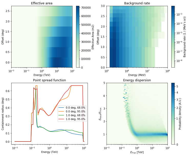
And also show a few overview plots using the .peek() method:
[9]:
analysis.observations["23592"].peek()
WARNING:gammapy.irf.psf_table:PSF does not integrate to unity within a precision of 1% in each energy bin. Containment radius computation might give biased results.
WARNING:gammapy.irf.psf_table:PSF does not integrate to unity within a precision of 1% in each energy bin. Containment radius computation might give biased results.
WARNING:gammapy.irf.psf_table:PSF does not integrate to unity within a precision of 1% in each energy bin. Containment radius computation might give biased results.
WARNING:gammapy.irf.psf_table:PSF does not integrate to unity within a precision of 1% in each energy bin. Containment radius computation might give biased results.
Data reduction
Now we proceed to the data reduction. In the config file we have chosen a WCS map geometry, energy axis and decided to stack the maps. We can run the reduction using .get_datasets():
[10]:
%%time
analysis.get_datasets()
INFO:gammapy.scripts.analysis:Creating geometry.
INFO:gammapy.scripts.analysis:Creating datasets.
CPU times: user 6.8 s, sys: 609 ms, total: 7.41 s
Wall time: 7.55 s
As we have chosen to stack the data, there is finally one dataset contained:
[11]:
analysis.datasets.names
[11]:
['stacked']
We can print the dataset as well:
[12]:
print(analysis.datasets["stacked"])
MapDataset

    Name                            : stacked

    Total counts                    : 7474
    Total predicted counts          : 2326.93
    Total background counts         : 2326.93

    Exposure min                    : 5.97e+07 m2 s
    Exposure max                    : 3.15e+09 m2 s

    Number of total bins            : 312500
    Number of fit bins              : 309230

    Fit statistic type              : cash
    Fit statistic value (-2 log(L)) : 73346.62

    Number of models                : 0
    Number of parameters            : 3
    Number of free parameters       : 1

    Component 0:
        Name                        : background
        Type                        : BackgroundModel
        Parameters:
            norm                    : 1.000
            tilt         (frozen)   : 0.000
            reference    (frozen)   : 1.000  TeV
As you can see the dataset comes with a predefined background model out of the data reduction, but no source model has been set yet.
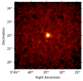
The counts, exposure and background model maps are directly available on the dataset and can be printed and plotted:
[13]:
counts = analysis.datasets["stacked"].counts
[14]:
print(counts)
WcsNDMap

        geom  : WcsGeom
        axes  : ['lon', 'lat', 'energy']
        shape : (250, 250, 5)
        ndim  : 3
        unit  :
        dtype : float32
[15]:
counts.smooth("0.05 deg").plot_interactive()
Model fitting
Now we define a model to be fitted to the dataset:
[16]:
model_config = """
components:
- name: crab
  type: SkyModel
  spatial:
    type: PointSpatialModel
    frame: icrs
    parameters:
    - name: lon_0
      value: 83.63
      unit: deg
    - name: lat_0
      value: 22.14
      unit: deg
  spectral:
    type: PowerLawSpectralModel
    parameters:
    - name: amplitude
      value: 1.0e-12
      unit: cm-2 s-1 TeV-1
    - name: index
      value: 2.0
      unit: ''
    - name: reference
      value: 1.0
      unit: TeV
      frozen: true
"""
Now we set the model on the analysis object:
[17]:
analysis.set_model(model_config)
INFO:gammapy.scripts.analysis:Reading model.
INFO:gammapy.scripts.analysis:SkyModels

Component 0: SkyModel

Parameters:

           name     value   error      unit      min max frozen
        --------- --------- ----- -------------- --- --- ------
            lon_0 8.363e+01   nan            deg nan nan  False
            lat_0 2.214e+01   nan            deg nan nan  False
        amplitude 1.000e-12   nan cm-2 s-1 TeV-1 nan nan  False
            index 2.000e+00   nan                nan nan  False
        reference 1.000e+00   nan            TeV nan nan   True
[18]:
print(analysis.model)
SkyModels

Component 0: SkyModel

Parameters:

           name     value   error      unit      min max frozen
        --------- --------- ----- -------------- --- --- ------
            lon_0 8.363e+01   nan            deg nan nan  False
            lat_0 2.214e+01   nan            deg nan nan  False
        amplitude 1.000e-12   nan cm-2 s-1 TeV-1 nan nan  False
            index 2.000e+00   nan                nan nan  False
        reference 1.000e+00   nan            TeV nan nan   True
[19]:
print(analysis.model["crab"])
SkyModel

Parameters:

           name     value   error      unit      min max frozen
        --------- --------- ----- -------------- --- --- ------
            lon_0 8.363e+01   nan            deg nan nan  False
            lat_0 2.214e+01   nan            deg nan nan  False
        amplitude 1.000e-12   nan cm-2 s-1 TeV-1 nan nan  False
            index 2.000e+00   nan                nan nan  False
        reference 1.000e+00   nan            TeV nan nan   True
Finally we run the fit:
[20]:
analysis.run_fit()
INFO:gammapy.scripts.analysis:Fitting reduced datasets.
INFO:gammapy.scripts.analysis:OptimizeResult

        backend    : minuit
        method     : minuit
        success    : True
        message    : Optimization terminated successfully.
        nfev       : 312
        total stat : 64490.20
[21]:
print(analysis.fit_result)
OptimizeResult

        backend    : minuit
        method     : minuit
        success    : True
        message    : Optimization terminated successfully.
        nfev       : 312
        total stat : 64490.20
This is how we can write the model back to file again:
[22]:
analysis.model.to_yaml("model-best-fit.yaml")
[23]:
!cat model-best-fit.yaml
components:
- name: crab
  type: SkyModel
  spatial:
    type: PointSpatialModel
    frame: icrs
    parameters:
    - name: lon_0
      value: 83.61894929306811
      unit: deg
    - name: lat_0
      value: 22.024836258944713
      unit: deg
  spectral:
    type: PowerLawSpectralModel
    parameters:
    - name: amplitude
      value: 6.290310266334393e-11
      unit: cm-2 s-1 TeV-1
    - name: index
      value: 2.785083946374748
      unit: ''
    - name: reference
      value: 1.0
      unit: TeV
      frozen: true
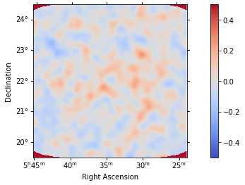
Inspecting residuals
For any fit it is usefull to inspect the residual images. We have a few option on the dataset object to handle this. First we can use .plot_residuals() to plot a residual image, summed over all energies:
[24]:
analysis.datasets["stacked"].plot_residuals(
    method="diff/sqrt(model)", vmin=-0.5, vmax=0.5
);
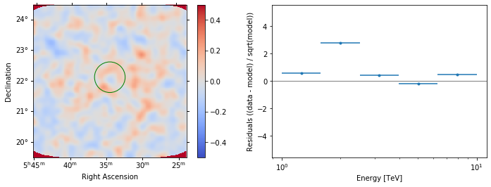
In addition we can aslo specify a region in the map to show the spectral residuals:
[25]:
region = CircleSkyRegion(
    center=SkyCoord("83.63 deg", "22.14 deg"), radius=0.5 * u.deg
)
[26]:
analysis.datasets["stacked"].plot_residuals(
    region=region, method="diff/sqrt(model)", vmin=-0.5, vmax=0.5
);
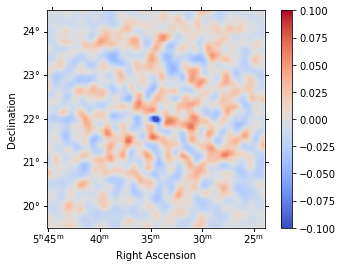
We can also directly access the .residuals() to get a map, that we can plot interactively:
[27]:
residuals = analysis.datasets["stacked"].residuals(method="diff")
residuals.smooth("0.08 deg").plot_interactive(
    cmap="coolwarm", vmin=-0.1, vmax=0.1, stretch="linear", add_cbar=True
)
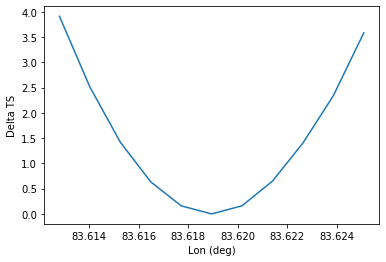
Inspecting likelihood profiles
To check the quality of the fit it is also useful to plot likelihood profiles for specific parameters. For this we use analysis.fit.likelihood_profile()
[28]:
profile = analysis.fit.likelihood_profile(parameter="lon_0")
For a good fit and error estimate the profile should be parabolic, if we plot it:
[29]:
total_stat = analysis.fit_result.total_stat
plt.plot(profile["values"], profile["likelihood"] - total_stat)
plt.xlabel("Lon (deg)")
plt.ylabel("Delta TS")
[29]:
Text(0, 0.5, 'Delta TS')
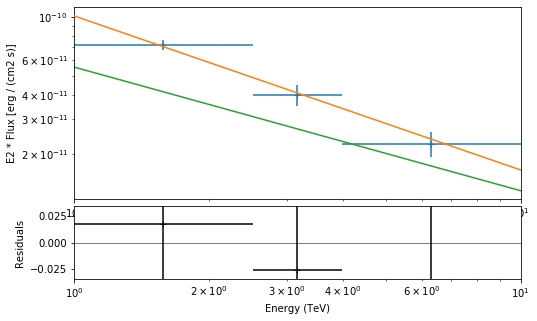
Flux points
[30]:
analysis.get_flux_points(source="crab")
INFO:gammapy.scripts.analysis:Calculating flux points.
INFO:gammapy.scripts.analysis:
      e_ref               ref_flux        ...        dnde_err        is_ul
       TeV              1 / (cm2 s)       ...    1 / (cm2 s TeV)
------------------ ---------------------- ... ---------------------- -----
1.5848931924611136 2.8430798565965568e-11 ... 1.0462744900578112e-12 False
3.1622776601683795  3.815367550602265e-12 ...  3.028947216617177e-13 False
 6.309573444801933 2.4140079194837277e-12 ...  4.951361673757777e-14 False
[31]:
plt.figure(figsize=(8, 5))
ax_sed, ax_residuals = analysis.flux_points.peek()
crab_spectrum = create_crab_spectral_model("hess_pl")
crab_spectrum.plot(
    ax=ax_sed,
    energy_range=[1, 10] * u.TeV,
    energy_power=2,
    flux_unit="erg-1 cm-2 s-1",
)
[31]:
<matplotlib.axes._subplots.AxesSubplot at 0x1289576d8>
Exercises
- Run a spectral analysis using reflected regions without stacking the datasets. You can use
AnalysisConfig.from_template("1d")to get an example configuration file. Add the resulting flux points to the SED plotted above.