This is a fixed-text formatted version of a Jupyter notebook
- Try online

- You can contribute with your own notebooks in this GitHub repository.
- Source files: image_fitting_with_sherpa.ipynb | image_fitting_with_sherpa.py
Fitting 2D images with Sherpa
Introduction
Sherpa is the X-ray satellite Chandra modeling and fitting application. It enables the user to construct complex models from simple definitions and fit those models to data, using a variety of statistics and optimization methods. The issues of constraining the source position and morphology are common in X- and Gamma-ray astronomy. This notebook will show you how to apply Sherpa to CTA data.
Here we will set up Sherpa to fit the counts map and loading the ancillary images for subsequent use. A relevant test statistic for data with Poisson fluctuations is the one proposed by Cash (1979). The simplex (or Nelder-Mead) fitting algorithm is a good compromise between efficiency and robustness. The source fit is best performed in pixel coordinates.
This tutorial has 2 important parts 1. Generating the Maps 2. The actual fitting with sherpa.
Since sherpa deals only with 2-dim images, the first part of this tutorial shows how to prepare gammapy maps to make classical images.
Necessary imports
[1]:
%matplotlib inline
import matplotlib.pyplot as plt
from pathlib import Path
import numpy as np
from astropy.io import fits
import astropy.units as u
from astropy.coordinates import SkyCoord
from gammapy.data import DataStore
from gammapy.irf import make_mean_psf
from gammapy.maps import WcsGeom, MapAxis, Map
from gammapy.cube import MapMaker, PSFKernel
1. Generating the required Maps
We first generate the required maps using 3 simulated runs on the Galactic center, exactly as in the analysis_3d tutorial.
It is always advisable to make the maps on fine energy bins, and then sum them over to get an image.
[2]:
# Define which data to use
data_store = DataStore.from_dir("$GAMMAPY_DATA/cta-1dc/index/gps/")
obs_ids = [110380, 111140, 111159]
observations = data_store.get_observations(obs_ids)
[3]:
energy_axis = MapAxis.from_edges(
    np.logspace(-1, 1.0, 10), unit="TeV", name="energy", interp="log"
)
geom = WcsGeom.create(
    skydir=(0, 0),
    binsz=0.02,
    width=(10, 8),
    coordsys="GAL",
    proj="CAR",
    axes=[energy_axis],
)
[4]:
%%time
maker = MapMaker(geom, offset_max=4.0 * u.deg)
maps = maker.run(observations)
WARNING: Tried to get polar motions for times after IERS data is valid. Defaulting to polar motion from the 50-yr mean for those. This may affect precision at the 10s of arcsec level [astropy.coordinates.builtin_frames.utils]
/Users/adonath/github/adonath/gammapy/gammapy/utils/interpolation.py:159: Warning: Interpolated values reached float32 precision limit
  "Interpolated values reached float32 precision limit", Warning
CPU times: user 13.4 s, sys: 2.54 s, total: 15.9 s
Wall time: 16 s
Making a PSF Map
Make a PSF map and weigh it with the exposure at the source position to get a 2D PSF
[5]:
# mean PSF
src_pos = SkyCoord(0, 0, unit="deg", frame="galactic")
table_psf = make_mean_psf(observations, src_pos)

# PSF kernel used for the model convolution
psf_kernel = PSFKernel.from_table_psf(table_psf, geom, max_radius="0.3 deg")

# get the exposure at the source position
exposure_at_pos = maps["exposure"].get_by_coord(
    {
        "lon": src_pos.l.value,
        "lat": src_pos.b.value,
        "energy": energy_axis.center,
    }
)

# now compute the 2D PSF
psf2D = psf_kernel.make_image(exposures=exposure_at_pos)
Make 2D images from 3D ones
Since sherpa image fitting works only with 2-dim images, we convert the generated maps to 2D images using run_images() and save them as fits files. The exposure is weighed with the spectrum before averaging (assumed to be a power law by default).
[6]:
maps = maker.run_images()
[7]:
Path("analysis_3d").mkdir(exist_ok=True)

maps["counts"].write("analysis_3d/counts_2D.fits", overwrite=True)
maps["background"].write("analysis_3d/background_2D.fits", overwrite=True)
maps["exposure"].write("analysis_3d/exposure_2D.fits", overwrite=True)
fits.writeto("analysis_3d/psf_2D.fits", psf2D.data, overwrite=True)
2. Analysis using sherpha
Read the maps and store them in a sherpa model
We now have the prepared files which sherpa can read. This part of the notebook shows how to do image analysis using sherpa
[8]:
import sherpa.astro.ui as sh

sh.set_stat("cash")
sh.set_method("simplex")

sh.load_image("analysis_3d/counts_2D.fits")
sh.set_coord("logical")

sh.load_table_model("expo", "analysis_3d/exposure_2D.fits")
sh.load_table_model("bkg", "analysis_3d/background_2D.fits")
sh.load_psf("psf", "analysis_3d/psf_2D.fits")
WARNING: imaging routines will not be available,
failed to import sherpa.image.ds9_backend due to
'RuntimeErr: DS9Win unusable: Could not find ds9 on your PATH'
WARNING: failed to import sherpa.astro.xspec; XSPEC models will not be available
To speed up this tutorial, we change the fit optimazation method to Levenberg-Marquardt and fix a required tolerance. This can make the fitting less robust, and in practise, you can skip this step unless you understand what is going on.
[9]:
sh.set_method("levmar")
sh.set_method_opt("xtol", 1e-5)
sh.set_method_opt("ftol", 1e-5)
sh.set_method_opt("gtol", 1e-5)
sh.set_method_opt("epsfcn", 1e-5)
[10]:
print(sh.get_method())
name    = levmar
ftol    = 1e-05
xtol    = 1e-05
gtol    = 1e-05
maxfev  = None
epsfcn  = 1e-05
factor  = 100.0
verbose = 0
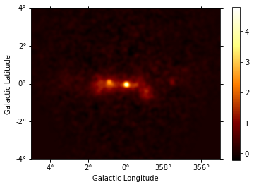
In principle one might first want to fit the background amplitude. However the background estimation method already yields the correct normalization, so we freeze the background amplitude to unity instead of adjusting it. The (smoothed) residuals from this background model are then computed and shown.
[11]:
sh.set_full_model(bkg)
bkg.ampl = 1
sh.freeze(bkg)
[12]:
resid = Map.read("analysis_3d/counts_2D.fits")
resid.data = sh.get_data_image().y - sh.get_model_image().y
resid_smooth = resid.smooth(width=4)
resid_smooth.plot(add_cbar=True);
Find and fit the brightest source
We then find the position of the maximum in the (smoothed) residuals map, and fit a (symmetrical) Gaussian source with that initial position:
[13]:
yp, xp = np.unravel_index(
    np.nanargmax(resid_smooth.data), resid_smooth.data.shape
)
ampl = resid_smooth.get_by_pix((xp, yp))[0]

# creates g0 as a gauss2d instance
sh.set_full_model(bkg + psf(sh.gauss2d.g0) * expo)
g0.xpos, g0.ypos = xp, yp
sh.freeze(g0.xpos, g0.ypos)  # fix the position in the initial fitting step

# fix exposure amplitude so that typical exposure is of order unity
expo.ampl = 1e-9
sh.freeze(expo)
sh.thaw(g0.fwhm, g0.ampl)  # in case frozen in a previous iteration

g0.fwhm = 10  # give some reasonable initial values
g0.ampl = ampl
[14]:
%%time
sh.fit()
/Users/adonath/software/anaconda3/envs/gammapy-dev/lib/python3.7/site-packages/sherpa/instrument.py:723: UserWarning: No PSF pixel size info available. Skipping check against data pixel size.
  warnings.warn("No PSF pixel size info available. Skipping check against data pixel size.")
Dataset               = 1
Method                = levmar
Statistic             = cash
Initial fit statistic = 291433
Final fit statistic   = 289598 at function evaluation 43
Data points           = 200000
Degrees of freedom    = 199998
Change in statistic   = 1834.33
   g0.fwhm        112.773      +/- 2.20899
   g0.ampl        0.441916     +/- 0.0126562
CPU times: user 1.95 s, sys: 29.2 ms, total: 1.98 s
Wall time: 1.99 s
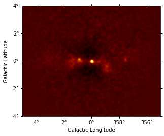
Fit all parameters of this Gaussian component, fix them and re-compute the residuals map.
[15]:
%%time
sh.thaw(g0.xpos, g0.ypos)
sh.fit()
sh.freeze(g0)
Dataset               = 1
Method                = levmar
Statistic             = cash
Initial fit statistic = 289598
Final fit statistic   = 289504 at function evaluation 26
Data points           = 200000
Degrees of freedom    = 199996
Change in statistic   = 94.5708
   g0.fwhm        107.444      +/- 2.10798
   g0.xpos        235.835      +/- 1.23177
   g0.ypos        195.201      +/- 1.28616
   g0.ampl        0.472507     +/- 0.0131969
CPU times: user 1.23 s, sys: 14 ms, total: 1.24 s
Wall time: 1.24 s
[16]:
resid.data = sh.get_data_image().y - sh.get_model_image().y
resid_smooth = resid.smooth(width=3)
resid_smooth.plot();
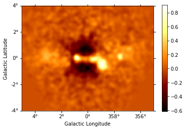
Iteratively find and fit additional sources
The residual map still shows the presence of additional components. Instantiate additional Gaussian components, and use them to iteratively fit sources, repeating the steps performed above for component g0. (The residuals map is shown after each additional source included in the model.) This would typically be done for many sources, but since this takes quite a bit of time, we demonstrate it for 3 iterations only here….
[17]:
# initialize components with fixed, zero amplitude
for i in range(1, 3):
    model = sh.create_model_component("gauss2d", "g" + str(i))
    model.ampl = 0
    sh.freeze(model)

sources = [g0, g1, g2]
sh.set_full_model(bkg + psf(g0 + g1 + g2) * expo)
[18]:
%%time
for gs in sources:
    yp, xp = np.unravel_index(
        np.nanargmax(resid_smooth.data), resid_smooth.data.shape
    )
    ampl = resid_smooth.get_by_pix((xp, yp))[0]
    gs.xpos, gs.ypos = xp, yp
    gs.fwhm = 10
    gs.ampl = ampl

    sh.thaw(gs.fwhm)
    sh.thaw(gs.ampl)
    sh.fit()

    sh.thaw(gs.xpos)
    sh.thaw(gs.ypos)
    sh.fit()
    sh.freeze(gs)

    resid.data = sh.get_data_image().y - sh.get_model_image().y
    resid_smooth = resid.smooth(width=6)
/Users/adonath/software/anaconda3/envs/gammapy-dev/lib/python3.7/site-packages/sherpa/instrument.py:723: UserWarning: No PSF pixel size info available. Skipping check against data pixel size.
  warnings.warn("No PSF pixel size info available. Skipping check against data pixel size.")
Dataset               = 1
Method                = levmar
Statistic             = cash
Initial fit statistic = 291453
Final fit statistic   = 289598 at function evaluation 43
Data points           = 200000
Degrees of freedom    = 199998
Change in statistic   = 1854.41
   g0.fwhm        112.768      +/- 2.20869
   g0.ampl        0.441937     +/- 0.0126579
Dataset               = 1
Method                = levmar
Statistic             = cash
Initial fit statistic = 289598
Final fit statistic   = 289504 at function evaluation 26
Data points           = 200000
Degrees of freedom    = 199996
Change in statistic   = 94.5716
   g0.fwhm        107.444      +/- 2.10798
   g0.xpos        235.835      +/- 1.23177
   g0.ypos        195.201      +/- 1.28615
   g0.ampl        0.472507     +/- 0.0131969
Dataset               = 1
Method                = levmar
Statistic             = cash
Initial fit statistic = 288955
Final fit statistic   = 288814 at function evaluation 20
Data points           = 200000
Degrees of freedom    = 199998
Change in statistic   = 140.418
   g1.fwhm        3.7736       +/- 0.479433
   g1.ampl        16.6573      +/- 3.64528
Dataset               = 1
Method                = levmar
Statistic             = cash
Initial fit statistic = 288814
Final fit statistic   = 288736 at function evaluation 22
Data points           = 200000
Degrees of freedom    = 199996
Change in statistic   = 78.7651
   g1.fwhm        2.20896      +/- 0.565577
   g1.xpos        253.097      +/- 0.182537
   g1.ypos        197.91       +/- 0.183642
   g1.ampl        46.2468      +/- 17.807
Dataset               = 1
Method                = levmar
Statistic             = cash
Initial fit statistic = 288519
Final fit statistic   = 288448 at function evaluation 10
Data points           = 200000
Degrees of freedom    = 199998
Change in statistic   = 70.7811
   g2.fwhm        19.6011      +/- 1.2746
   g2.ampl        0.958563     +/- 0.112208
Dataset               = 1
Method                = levmar
Statistic             = cash
Initial fit statistic = 288448
Final fit statistic   = 288330 at function evaluation 51
Data points           = 200000
Degrees of freedom    = 199996
Change in statistic   = 117.726
   g2.fwhm        35.4186      +/- 1.87188
   g2.xpos        187.112      +/- 1.11498
   g2.ypos        197.468      +/- 1.13358
   g2.ampl        0.59605      +/- 0.0505517
CPU times: user 8.83 s, sys: 82.4 ms, total: 8.91 s
Wall time: 8.91 s
[19]:
resid_smooth.plot(add_cbar=True);
Generating output table and Test Statistics estimation
When adding a new source, one needs to check the significance of this new source. A frequently used method is the Test Statistics (TS). This is done by comparing the change of statistics when the source is included compared to the null hypothesis (no source ; in practice here we fix the amplitude to zero).
\(TS = Cstat(source) - Cstat(no source)\)
The criterion for a significant source detection is typically that it should improve the test statistic by at least 25 or 30. We have added only 3 sources to save time, but you should keep doing this till del(stat) is less than the required number.
[20]:
from astropy.stats import gaussian_fwhm_to_sigma
from astropy.table import Table

rows = []
for g in sources:
    ampl = g.ampl.val
    g.ampl = 0
    stati = sh.get_stat_info()[0].statval
    g.ampl = ampl
    statf = sh.get_stat_info()[0].statval
    delstat = stati - statf

    geom = resid.geom
    # sherpa uses 1 based indexing
    coord = geom.pix_to_coord((g.xpos.val - 1, g.ypos.val - 1))
    pix_scale = geom.pixel_scales.mean().deg
    sigma = g.fwhm.val * pix_scale * gaussian_fwhm_to_sigma
    rows.append(
        dict(
            delstat=delstat,
            glon=coord[0].to_value("deg"),
            glat=coord[1].to_value("deg"),
            sigma=sigma,
        )
    )

table = Table(rows=rows, names=rows[0])
for name in table.colnames:
    table[name].format = ".5g"
/Users/adonath/software/anaconda3/envs/gammapy-dev/lib/python3.7/site-packages/sherpa/instrument.py:723: UserWarning: No PSF pixel size info available. Skipping check against data pixel size.
  warnings.warn("No PSF pixel size info available. Skipping check against data pixel size.")
[21]:
table
[21]:
| delstat | glon | glat | sigma |
|---|---|---|---|
| float64 | float64 | float64 | float64 |
| 1792.3 | 0.2933 | -0.10598 | 0.91255 |
| 768.04 | 359.95 | -0.051805 | 0.018761 |
| 405.36 | 1.2678 | -0.06064 | 0.30082 |
Exercises
- Keep adding sources till there are no more significat ones in the field. How many Gaussians do you need?
- Use other morphologies for the sources (eg: disk, shell) rather than only Gaussian.
- Compare the TS between different models
More about sherpa
These are good resources to learn more about Sherpa:
- https://python4astronomers.github.io/fitting/fitting.html
- https://github.com/DougBurke/sherpa-standalone-notebooks
You could read over the examples there, and try to apply a similar analysis to this dataset here to practice.
If you want a deeper understanding of how Sherpa works, then these proceedings are good introductions: