This is a fixed-text formatted version of a Jupyter notebook
- Try online

- You can contribute with your own notebooks in this GitHub repository.
- Source files: analysis_3d_joint.ipynb | analysis_3d_joint.py
Joint 3D Analysis
In this tutorial we show how to run a joint 3D map-based analysis using three example observations of the Galactic center region with CTA. We start with the required imports:
[1]:
%matplotlib inline
from matplotlib.patches import Circle
import numpy as np
[2]:
from pathlib import Path
from astropy import units as u
from astropy.coordinates import SkyCoord
[3]:
from gammapy.data import DataStore
from gammapy.irf import EnergyDispersion, make_psf
from gammapy.maps import WcsGeom, MapAxis, Map
from gammapy.cube import MapMaker, PSFKernel, MapDataset
from gammapy.cube.models import SkyModel, BackgroundModel
from gammapy.spectrum.models import PowerLaw
from gammapy.image.models import SkyPointSource
from gammapy.utils.fitting import Fit
Prepare modeling input data
We first use the DataStore object to access the CTA observations and retrieve a list of observations by passing the observations IDs to the .get_observations() method:
[4]:
# Define which data to use and print some information
data_store = DataStore.from_dir("$GAMMAPY_DATA/cta-1dc/index/gps/")
[5]:
# Select some observations from these dataset by hand
obs_ids = [110380, 111140, 111159]
observations = data_store.get_observations(obs_ids)
Prepare input maps
Now we define a reference geometry for our analysis, We choose a WCS based gemoetry with a binsize of 0.02 deg and also define an energy axis:
[6]:
energy_axis = MapAxis.from_edges(
    np.logspace(-1.0, 1.0, 10), unit="TeV", name="energy", interp="log"
)
geom = WcsGeom.create(
    skydir=(0, 0),
    binsz=0.02,
    width=(10, 8),
    coordsys="GAL",
    proj="CAR",
    axes=[energy_axis],
)
In addition we define the center coordinate and the FoV offset cut:
[7]:
# Source position
src_pos = SkyCoord(0, 0, unit="deg", frame="galactic")

# FoV max
offset_max = 4 * u.deg
The maps are prepared by calling the MapMaker.run() method and passing the observations. The .run() method returns a Python dict containing a counts, background and exposure map. For the joint analysis, we compute the cube per observation and store the result in the observations_maps dictionary.
[8]:
%%time
observations_data = {}

for obs in observations:
    # For each observation, the map will be centered on the pointing position.
    geom_cutout = geom.cutout(
        position=obs.pointing_radec, width=2 * offset_max
    )
    maker = MapMaker(geom_cutout, offset_max=offset_max)
    maps = maker.run([obs])
    observations_data[obs.obs_id] = maps
WARNING: Tried to get polar motions for times after IERS data is valid. Defaulting to polar motion from the 50-yr mean for those. This may affect precision at the 10s of arcsec level [astropy.coordinates.builtin_frames.utils]
CPU times: user 23.1 s, sys: 2.29 s, total: 25.4 s
Wall time: 22.9 s
Prepare IRFs
PSF and Edisp are estimated for each observation at a specific source position defined by src_pos:
[9]:
# define energy grid for edisp
energy = energy_axis.edges
[10]:
for obs in observations:
    table_psf = make_psf(obs, src_pos)
    psf = PSFKernel.from_table_psf(table_psf, geom, max_radius="0.5 deg")
    observations_data[obs.obs_id]["psf"] = psf

    # create Edisp
    offset = src_pos.separation(obs.pointing_radec)
    edisp = obs.edisp.to_energy_dispersion(
        offset, e_true=energy, e_reco=energy
    )
    observations_data[obs.obs_id]["edisp"] = edisp
Save maps as well as IRFs to disk:
[11]:
for obs_id in obs_ids:
    path = Path("analysis_3d_joint") / "obs_{}".format(obs_id)
    path.mkdir(parents=True, exist_ok=True)

    for key in ["counts", "exposure", "background", "edisp", "psf"]:
        filename = "{}.fits.gz".format(key)
        observations_data[obs_id][key].write(path / filename, overwrite=True)
Likelihood fit
Reading maps and IRFs
As first step we define a source model:
[12]:
spatial_model = SkyPointSource(lon_0="-0.05 deg", lat_0="-0.05 deg")
spectral_model = PowerLaw(
    index=2.4, amplitude="2.7e-12 cm-2 s-1 TeV-1", reference="1 TeV"
)
model = SkyModel(spatial_model=spatial_model, spectral_model=spectral_model)
Now we read the maps and IRFs and create the dataset for each observation:
[13]:
datasets = []

for obs_id in obs_ids:
    path = Path("analysis_3d_joint") / "obs_{}".format(obs_id)

    # read counts map and IRFs
    counts = Map.read(path / "counts.fits.gz")
    exposure = Map.read(path / "exposure.fits.gz")

    psf = PSFKernel.read(path / "psf.fits.gz")
    edisp = EnergyDispersion.read(path / "edisp.fits.gz")

    # create background model per observation / dataset
    background = Map.read(path / "background.fits.gz")
    background_model = BackgroundModel(background)
    background_model.tilt.frozen = False
    background_model.norm.value = 1.3

    # optionally define a safe energy threshold
    emin = None
    mask = counts.geom.energy_mask(emin=emin)

    dataset = MapDataset(
        model=model,
        counts=counts,
        exposure=exposure,
        psf=psf,
        edisp=edisp,
        background_model=background_model,
        mask_fit=mask,
    )

    datasets.append(dataset)
[14]:
fit = Fit(datasets)
[15]:
%%time
result = fit.run()
CPU times: user 56.9 s, sys: 3.53 s, total: 1min
Wall time: 31.3 s
[16]:
print(result)
OptimizeResult

        backend    : minuit
        method     : minuit
        success    : True
        message    : Optimization terminated successfully.
        nfev       : 409
        total stat : 922625.68
Best fit parameters:
[17]:
fit.datasets.parameters.to_table()
[17]:
| name | value | error | unit | min | max | frozen |
|---|---|---|---|---|---|---|
| str9 | float64 | float64 | str14 | float64 | float64 | bool |
| lon_0 | -5.248e-02 | 2.234e-03 | deg | -1.800e+02 | 1.800e+02 | False |
| lat_0 | -5.205e-02 | 2.131e-03 | deg | -9.000e+01 | 9.000e+01 | False |
| index | 2.366e+00 | 4.139e-02 | nan | nan | False | |
| amplitude | 2.667e-12 | 1.379e-13 | cm-2 s-1 TeV-1 | nan | nan | False |
| reference | 1.000e+00 | 0.000e+00 | TeV | nan | nan | True |
| norm | 1.311e+00 | 1.247e-02 | 0.000e+00 | nan | False | |
| tilt | -1.091e-01 | 5.800e-03 | nan | nan | False | |
| reference | 1.000e+00 | 0.000e+00 | TeV | nan | nan | True |
| norm | 1.310e+00 | 1.260e-02 | 0.000e+00 | nan | False | |
| tilt | -1.064e-01 | 5.852e-03 | nan | nan | False | |
| reference | 1.000e+00 | 0.000e+00 | TeV | nan | nan | True |
| norm | 1.324e+00 | 1.264e-02 | 0.000e+00 | nan | False | |
| tilt | -1.186e-01 | 5.819e-03 | nan | nan | False | |
| reference | 1.000e+00 | 0.000e+00 | TeV | nan | nan | True |
The information which parameter belongs to which dataset is not listed explicitely in the table (yet), but the order of parameters is conserved. You can always access the underlying object tree as well to get specific parameter values:
[18]:
for dataset in datasets:
    print(dataset.background_model.norm.value)
1.31074947621015
1.3095902784780802
1.3244160732022032
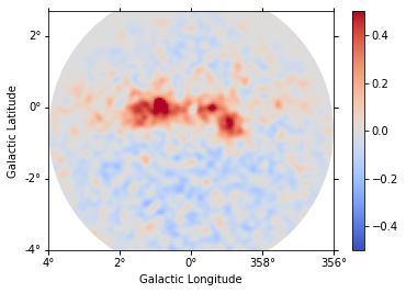
Plotting residuals
[19]:
def plot_residuals(dataset):
    npred = dataset.npred()
    residual = (dataset.counts - npred).sum_over_axes().smooth("0.08 deg")
    _, ax, _ = residual.plot(
        vmin=-0.5, vmax=0.5, cmap="coolwarm", add_cbar=True, stretch="linear"
    )
    x_center, y_center, _ = dataset.counts.geom.center_coord
    fov = Circle(
        (x_center, y_center), radius=4, transform=ax.get_transform("galactic")
    )
    ax.images[0].set_clip_path(fov)
Each observation has different energy threshold. Keep in mind that the residuals are not meaningful below the energy threshold.
[20]:
plot_residuals(datasets[0])
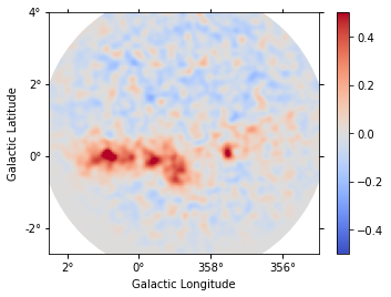
[21]:
plot_residuals(datasets[1])
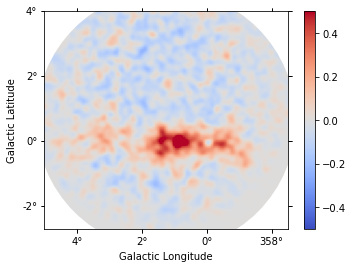
[22]:
plot_residuals(datasets[2])
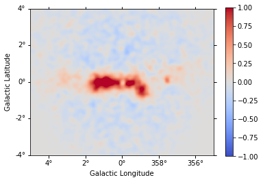
Finally we compute as stacked residual map (this requires to run the analysis_3d tutorial first):
[23]:
npred_stacked = Map.from_geom(geom)
counts_stacked = Map.from_geom(geom)

for dataset in datasets:
    npred = dataset.npred()
    coords = npred.geom.get_coord()

    npred_stacked.fill_by_coord(coords, npred.data)
    counts_stacked.fill_by_coord(coords, dataset.counts.data)
[24]:
residual_stacked = (
    (counts_stacked - npred_stacked).sum_over_axes().smooth("0.1 deg")
)
[25]:
residual_stacked.plot(
    vmin=-1, vmax=1, cmap="coolwarm", add_cbar=True, stretch="linear"
);
[26]: