Feldman and Cousins Confidence Intervals
Feldman and Cousins solved the problem on how to choose confidence intervals in
a unified way (that is without basing the choice on the data) [Feldman1998].
The functions gammapy.stats.fc_* give you access to a numerical solution to
the Feldman Cousins algorithm. It can be used for any type of statistical
distribution and is not limited to a Poisson process with background or a
Gaussian with a boundary at the origin.
The basic ingredient to fc_construct_acceptance_intervals_pdfs
is a matrix of \(P(X|\\mu)\) (see e.g. equation (3.1) and (3.2) in
[Feldman1998]). Every row is a probability density function (PDF) of x and the
columns are built up by varying the signal strength \(\\mu\). The other
parameter is the desired confidence level (C.L.). The function will return
another matrix of acceptance intervals where 1 means the point is part of the
acceptance interval and 0 means it is outside. This can be easily converted to
upper and lower limits (fc_get_limits), which simply connect
the outside 1s for different \(\\mu\) values. An upper or lower limit is
obtained by drawing a vertical line at the measured value and calculating the
intersection (fc_find_limit).
Examples
Assume you have a Poisson background with known mean 3.0. We generate the matrix of \(P(X|\\mu)\) like this
import gammapy.stats as gstats
import numpy as np
from scipy import stats

x_bins = np.arange(0, 50)
mu_bins = np.linspace(0, 15, 15 / 0.005 + 1, endpoint=True)
matrix = [stats.poisson(mu + 3.0).pmf(x_bins) for mu in mu_bins]
Now we generate the 90% acceptance intervals and construct the lower and upper limit from them:
acceptance_intervals = gstats.fc_construct_acceptance_intervals_pdfs(matrix, 0.9)
LowerLimitNum, UpperLimitNum, _ = gstats.fc_get_limits(mu_bins, x_bins, acceptance_intervals)
Let’s say you measured x = 1, then the 90% upper limit would be:
>>> gstats.fc_find_limit(1, UpperLimitNum, mu_bins)
1.875
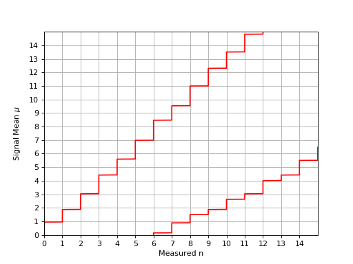
The following plot shows the confidence belt based on the Feldman and Cousins principle for a 90% confidence level for the unknown Poisson signal mean \(\\mu\). It is a reproduction of Fig. 7 from [Feldman1998]. It should be noted that the plot in the paper is inconsistent with Table IV from the same paper: the lower limit is off by one bin to the left.
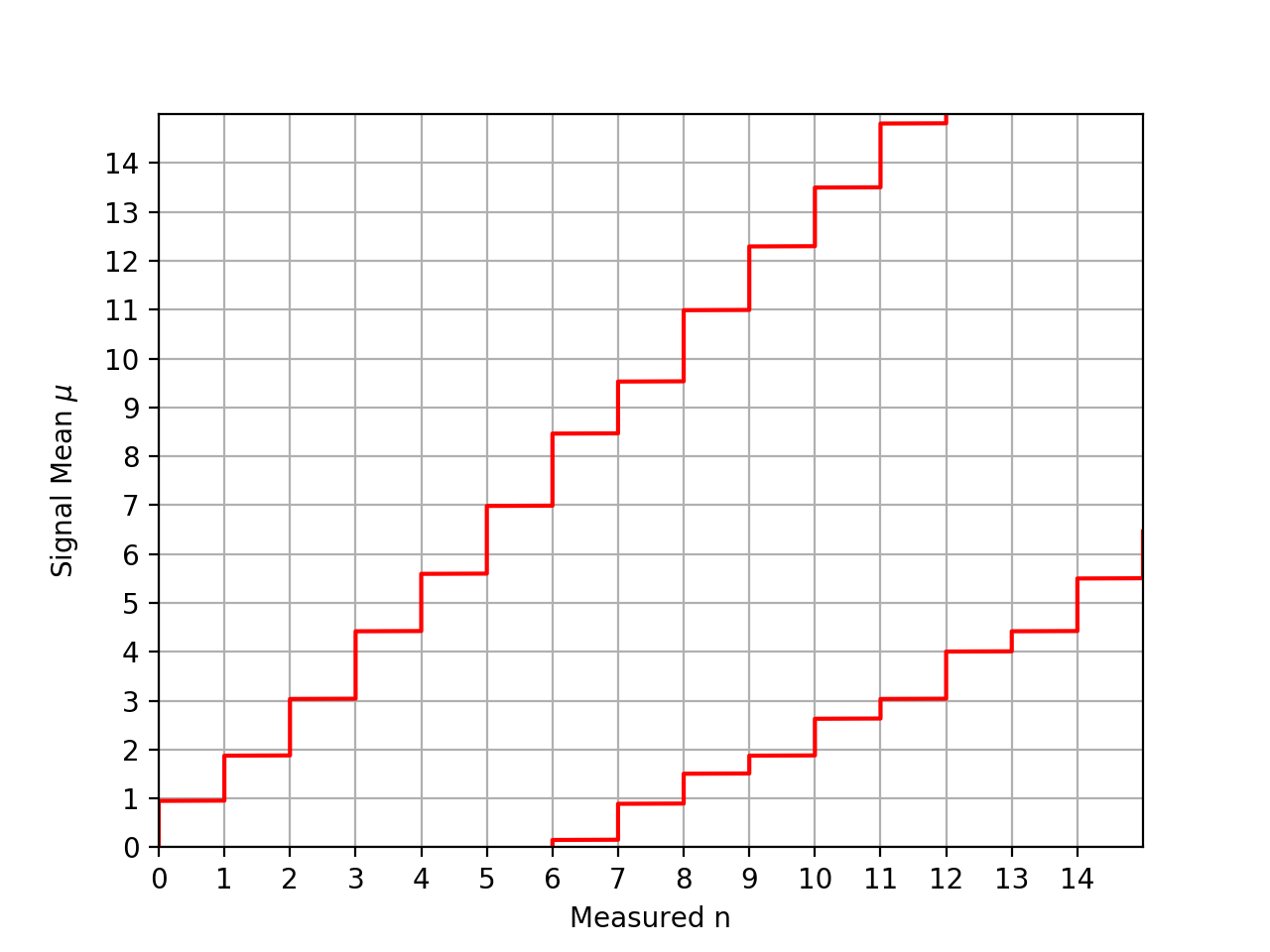
Assume you have an experiment where the observable x is simply the measured value of \(\\mu\) in an experiment with a Gaussian resolution with known width \(\\sigma\). The following plot shows the confidence belt based on the Feldman and Cousins principle for a 90% confidence level for the mean of the Gaussian \(\\mu\), constrained to be non-negative. it reproduces Fig. 10 from [Feldman1998].
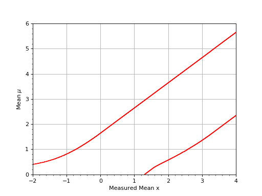
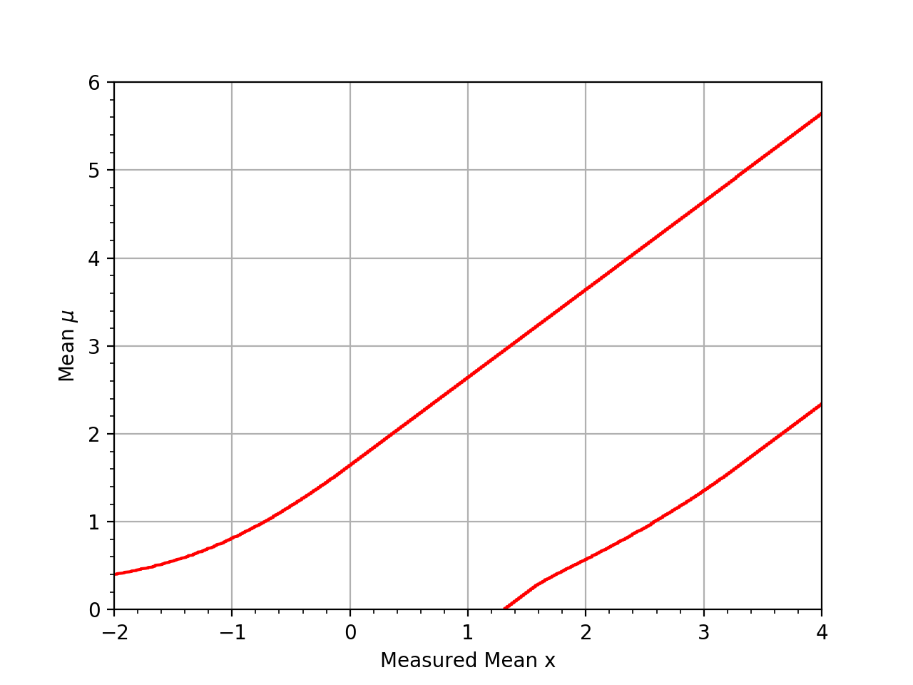

Acceptance Interval Fixing
Feldman and Cousins point out that sometimes the set of intersected horizontal
lines is not simply connected. These artefacts are corrected with
fc_fix_limits.
>>> gstats.fc_fix_limits(LowerLimitNum, UpperLimitNum)
The following script in the examples directory demonstrates the problem:
example_fc_demonstrate_artefact.py
For mu = 0.745 the 90% acceptance interval is [0,8] and for mu = 0.750 it is
[1,8]. A lot of the fast algorithms that do not compute the full confidence belt
will come to the conclusion that the 90% confidence interval is [0, 0.745] and
thus the upper limit when zero is measured should be 0.745 (one example is
TFeldmanCousins that comes with ROOT, but is has the additional bug of
making the confidence interval one mu bin to big, thus reporting 0.75 as upper
limit).
For mu = 1.035 the 90% acceptance interval is [0,8] again and only starting mu = 1.060 will 0 no longer be in the 90% acceptance interval. Thus the correct upper limit according to the procedure described in [Feldman1998] should be 1.055, which is also the value given in the paper (rounded to 1.06).
Sensitivity
[Feldman1998] also defines experimental sensitivity as the average upper limit
that would be obtained by an ensemble of experiments with the expected
background and no true signal. It can be calculated using
fc_find_average_upper_limit.
>>> gstats.fc_find_average_upper_limit(x_bins, matrix, UpperLimitNum, mu_bins)
4.41
General Case
In the more general case, one may not know the underlying PDF of
\(P(X|\\mu)\). One way would be to generate \(P(X|\\mu)\) from Monte
Carlo simulation. With a dictionary of mu values and lists of X values from
Monte Carlo one can use fc_construct_acceptance_intervals to
construct the confidence belts.
Here is an example, where the X values are generated from Monte Carlo (seed is fixed here, so the result is known):
import gammapy.stats as gstats
import numpy as np
from scipy import stats

x_bins = np.linspace(-10, 10, 100, endpoint=True)
mu_bins = np.linspace(0, 8, 8 / 0.05 + 1, endpoint=True)

np.random.seed(seed=1)

distribution_dict = dict((mu, [stats.norm.rvs(loc=mu, scale=1, size=5000)]) for mu in mu_bins)

acceptance_intervals = gstats.fc_construct_acceptance_intervals(distribution_dict, x_bins, 0.6827)

LowerLimitNum, UpperLimitNum, _ = gstats.fc_get_limits(mu_bins, x_bins, acceptance_intervals)

mu_upper_limit = gstats.fc_find_limit(1.7, UpperLimitNum, mu_bins)
# mu_upper_limit == 2.7
Verification
To verify that the numerical solution is working, the example plots can also be
produced using the analytical solution. They look consistent. The scripts for
the analytical solution are given in the examples directory:
example_fc_poisson_analytical.py
example_fc_gauss_analytical.py