This is a fixed-text formatted version of a Jupyter notebook
- Try online

- You can contribute with your own notebooks in this GitHub repository.
- Source files: detect_ts.ipynb | detect_ts.py
Source detection with Gammapy
Introduction
This notebook show how to do source detection with Gammapy using one of the methods available in gammapy.detect.
We will do this:
- produce 2-dimensional test-statistics (TS) images using Fermi-LAT 3FHL high-energy Galactic center dataset
- run a peak finder to make a source catalog
- do some simple measurements on each source
- compare to the 3FHL catalog
Note that what we do here is a quick-look analysis, the production of real source catalogs use more elaborate procedures.
We will work with the following functions and classes:
Setup
As always, let’s get started with some setup …
[1]:
%matplotlib inline
import matplotlib.pyplot as plt
[2]:
from gammapy.maps import Map
from gammapy.detect import TSMapEstimator, find_peaks
from gammapy.catalog import source_catalogs
from gammapy.cube import PSFKernel
Read in input images
We first read in the counts cube and sum over the energy axis:
[3]:
counts = Map.read("$GAMMAPY_DATA/fermi-3fhl-gc/fermi-3fhl-gc-counts.fits.gz")
background = Map.read(
    "$GAMMAPY_DATA/fermi-3fhl-gc/fermi-3fhl-gc-background.fits.gz"
)
exposure = Map.read(
    "$GAMMAPY_DATA/fermi-3fhl-gc/fermi-3fhl-gc-exposure.fits.gz"
)

maps = {"counts": counts, "background": background, "exposure": exposure}

kernel = PSFKernel.read(
    "$GAMMAPY_DATA/fermi-3fhl-gc/fermi-3fhl-gc-psf.fits.gz"
)
[4]:
%%time
estimator = TSMapEstimator()
images = estimator.run(maps, kernel.data)
CPU times: user 948 ms, sys: 97.1 ms, total: 1.05 s
Wall time: 10.8 s
Plot images
[5]:
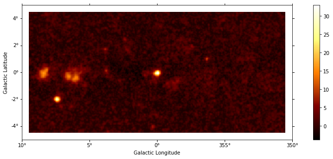
plt.figure(figsize=(15, 5))
images["sqrt_ts"].plot(add_cbar=True);
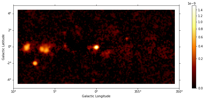
[6]:
plt.figure(figsize=(15, 5))
images["flux"].plot(add_cbar=True, stretch="sqrt", vmin=0);
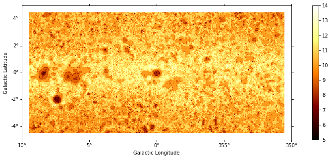
[7]:
plt.figure(figsize=(15, 5))
images["niter"].plot(add_cbar=True);
Source catalog
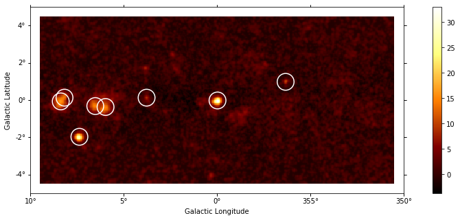
Let’s run a peak finder on the sqrt_ts image to get a list of sources (positions and peak sqrt_ts values).
[8]:
sources = find_peaks(images["sqrt_ts"], threshold=8)
sources
[8]:
| value | x | y | ra | dec |
|---|---|---|---|---|
| deg | deg | |||
| float64 | int64 | int64 | float64 | float64 |
| 32.972 | 200 | 99 | 266.41449 | -28.97054 |
| 27.995 | 52 | 60 | 272.43197 | -23.54282 |
| 16.18 | 32 | 98 | 271.16056 | -21.74479 |
| 14.939 | 69 | 93 | 270.40919 | -23.47797 |
| 14.842 | 80 | 92 | 270.15899 | -23.98049 |
| 13.951 | 36 | 102 | 270.86716 | -21.82076 |
| 9.7245 | 273 | 119 | 263.18257 | -31.52587 |
| 8.8532 | 124 | 102 | 268.46711 | -25.63326 |
[9]:
# Plot sources on top of significance sky image
plt.figure(figsize=(15, 5))

_, ax, _ = images["sqrt_ts"].plot(add_cbar=True)

ax.scatter(
    sources["ra"],
    sources["dec"],
    transform=plt.gca().get_transform("icrs"),
    color="none",
    edgecolor="w",
    marker="o",
    s=600,
    lw=1.5,
);
Measurements
- TODO: show cutout for a few sources and some aperture photometry measurements (e.g. energy distribution, significance, flux)
[10]:
# TODO
Compare to 3FHL
TODO
[11]:
fermi_3fhl = source_catalogs["3fhl"]
[12]:
selection = counts.geom.contains(fermi_3fhl.positions)
fermi_3fhl.table = fermi_3fhl.table[selection]
[13]:
fermi_3fhl.table[["Source_Name", "GLON", "GLAT"]]
[13]:
| Source_Name | GLON | GLAT |
|---|---|---|
| deg | deg | |
| bytes18 | float32 | float32 |
| 3FHL J1731.7-3003 | 357.4511 | 1.9489 |
| 3FHL J1732.6-3131 | 356.3192 | 0.9981 |
| 3FHL J1741.8-2536 | 2.3923 | 2.4610 |
| 3FHL J1744.5-2609 | 2.2387 | 1.6537 |
| 3FHL J1745.6-2900 | 359.9423 | -0.0497 |
| 3FHL J1745.8-3028e | 358.7080 | -0.8370 |
| 3FHL J1746.2-2852 | 0.1225 | -0.0882 |
| 3FHL J1747.2-2959 | 359.2745 | -0.8456 |
| 3FHL J1747.2-2822 | 0.6775 | -0.0182 |
| ... | ... | ... |
| 3FHL J1753.8-2537 | 3.7706 | 0.1398 |
| 3FHL J1800.5-2343e | 6.1952 | -0.2333 |
| 3FHL J1800.7-2357 | 6.0099 | -0.3812 |
| 3FHL J1801.5-2450 | 5.3311 | -0.9750 |
| 3FHL J1801.6-2327 | 6.5336 | -0.3132 |
| 3FHL J1802.3-3043 | 0.2988 | -4.0414 |
| 3FHL J1803.1-2148 | 8.1470 | 0.1906 |
| 3FHL J1804.7-2144e | 8.3974 | -0.0948 |
| 3FHL J1809.8-2332 | 7.3904 | -1.9952 |
| 3FHL J1811.2-2800 | 3.6168 | -4.4098 |
What next?
In this notebook, we have seen how to work with images and compute TS images from counts data, if a background estimate is already available.
Here’s some suggestions what to do next:
- TODO: point to background estimation examples
- TODO: point to other docs …