This is a fixed-text formatted version of a Jupyter notebook

Try online
You can contribute with your own notebooks in this GitHub repository.
Source files: sed_fitting_gammacat_fermi.ipynb | sed_fitting_gammacat_fermi.py

Flux point fitting in Gammapy¶

Introduction¶

In this tutorial we’re going to learn how to fit spectral models to combined Fermi-LAT and IACT flux points.

The central class we’re going to use for this example analysis is:

gammapy.spectrum.FluxPointsDataset

In addition we will work with the following data classes:

And the following spectral model classes:

Setup¶

Let us start with the usual IPython notebook and Python imports:

[1]:

%matplotlib inline
import numpy as np
import matplotlib.pyplot as plt

[2]:

from astropy import units as u
from gammapy.spectrum.models import (
    PowerLaw,
    ExponentialCutoffPowerLaw,
    LogParabola,
)
from gammapy.spectrum import FluxPointsDataset, FluxPoints
from gammapy.catalog import (
    SourceCatalog3FGL,
    SourceCatalogGammaCat,
    SourceCatalog3FHL,
)
from gammapy.utils.fitting import Fit

Load spectral points¶

For this analysis we choose to work with the source ‘HESS J1507-622’ and the associated Fermi-LAT sources ‘3FGL J1506.6-6219’ and ‘3FHL J1507.9-6228e’. We load the source catalogs, and then access source of interest by name:

[3]:

fermi_3fgl = SourceCatalog3FGL()
fermi_3fhl = SourceCatalog3FHL()
gammacat = SourceCatalogGammaCat("$GAMMAPY_DATA/gamma-cat/gammacat.fits.gz")

[4]:

source_gammacat = gammacat["HESS J1507-622"]
source_fermi_3fgl = fermi_3fgl["3FGL J1506.6-6219"]
source_fermi_3fhl = fermi_3fhl["3FHL J1507.9-6228e"]

The corresponding flux points data can be accessed with .flux_points attribute:

[5]:

flux_points_gammacat = source_gammacat.flux_points
flux_points_gammacat.table

[5]:

Table length=6

e_ref	dnde	dnde_errn	dnde_errp
TeV	1 / (cm2 s TeV)	1 / (cm2 s TeV)	1 / (cm2 s TeV)
float32	float32	float32	float32
0.8609004	2.29119e-12	8.705427e-13	8.955021e-13
1.561512	6.981717e-13	2.203541e-13	2.304066e-13
2.763753	1.690615e-13	6.758698e-14	7.188384e-14
4.891597	7.729249e-14	2.401318e-14	2.607487e-14
9.988584	1.032534e-14	5.063147e-15	5.641954e-15
27.04035	7.449867e-16	5.72089e-16	7.259987e-16

In the Fermi-LAT catalogs, integral flux points are given. Currently the flux point fitter only works with differential flux points, so we apply the conversion here.

[6]:

flux_points_3fgl = source_fermi_3fgl.flux_points.to_sed_type(
    sed_type="dnde", model=source_fermi_3fgl.spectral_model
)
flux_points_3fhl = source_fermi_3fhl.flux_points.to_sed_type(
    sed_type="dnde", model=source_fermi_3fhl.spectral_model
)

Finally we stack the flux points into a single FluxPoints object and drop the upper limit values, because currently we can’t handle them in the fit:

[7]:

# stack flux point tables
flux_points = FluxPoints.stack(
    [flux_points_gammacat, flux_points_3fhl, flux_points_3fgl]
)

# drop the flux upper limit values
flux_points = flux_points.drop_ul()

Power Law Fit¶

First we start with fitting a simple power law.

[8]:

pwl = PowerLaw(index=2, amplitude="1e-12 cm-2 s-1 TeV-1", reference="1 TeV")

After creating the model we run the fit by passing the 'flux_points' and 'pwl' objects:

[9]:

dataset_pwl = FluxPointsDataset(pwl, flux_points, likelihood="chi2assym")
fitter = Fit(dataset_pwl)
result_pwl = fitter.run()

And print the result:

[10]:

print(result_pwl)

OptimizeResult

        backend    : minuit
        method     : minuit
        success    : True
        message    : Optimization terminated successfully.
        nfev       : 40
        total stat : 33.68

[11]:

print(pwl)

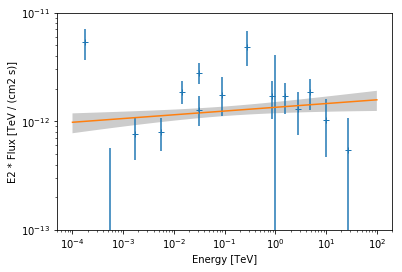
PowerLaw

Parameters:

           name     value   error      unit      min max frozen
        --------- --------- ----- -------------- --- --- ------
            index 1.966e+00   nan                nan nan  False
        amplitude 1.345e-12   nan cm-2 s-1 TeV-1 nan nan  False
        reference 1.000e+00   nan            TeV nan nan   True

Finally we plot the data points and the best fit model:

[12]:

ax = flux_points.plot(energy_power=2)
pwl.plot(energy_range=[1e-4, 1e2] * u.TeV, ax=ax, energy_power=2)

# assign covariance for plotting
pwl.parameters.covariance = result_pwl.parameters.covariance

pwl.plot_error(energy_range=[1e-4, 1e2] * u.TeV, ax=ax, energy_power=2)
ax.set_ylim(1e-13, 1e-11);

../_images/notebooks_sed_fitting_gammacat_fermi_22_0.png

Exponential Cut-Off Powerlaw Fit¶

Next we fit an exponential cut-off power law to the data.

[13]:

ecpl = ExponentialCutoffPowerLaw(
    index=1.8,
    amplitude="2e-12 cm-2 s-1 TeV-1",
    reference="1 TeV",
    lambda_="0.1 TeV-1",
)

We run the fitter again by passing the flux points and the ecpl model instance:

[14]:

dataset_ecpl = FluxPointsDataset(ecpl, flux_points, likelihood="chi2assym")
fitter = Fit(dataset_ecpl)
result_ecpl = fitter.run()
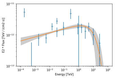
print(ecpl)

ExponentialCutoffPowerLaw

Parameters:

           name     value   error      unit      min max frozen
        --------- --------- ----- -------------- --- --- ------
            index 1.869e+00   nan                nan nan  False
        amplitude 2.126e-12   nan cm-2 s-1 TeV-1 nan nan  False
        reference 1.000e+00   nan            TeV nan nan   True
          lambda_ 1.000e-01   nan          TeV-1 nan nan  False

We plot the data and best fit model:

[15]:

ax = flux_points.plot(energy_power=2)
ecpl.plot(energy_range=[1e-4, 1e2] * u.TeV, ax=ax, energy_power=2)

# assign covariance for plotting
ecpl.parameters.covariance = result_ecpl.parameters.covariance

ecpl.plot_error(energy_range=[1e-4, 1e2] * u.TeV, ax=ax, energy_power=2)
ax.set_ylim(1e-13, 1e-11)

[15]:

(1e-13, 1e-11)

../_images/notebooks_sed_fitting_gammacat_fermi_28_1.png

Log-Parabola Fit¶

Finally we try to fit a log-parabola model:

[16]:

log_parabola = LogParabola(
    alpha=2, amplitude="1e-12 cm-2 s-1 TeV-1", reference="1 TeV", beta=0.1
)

[17]:

dataset_log_parabola = FluxPointsDataset(
    log_parabola, flux_points, likelihood="chi2assym"
)
fitter = Fit(dataset_log_parabola)
result_log_parabola = fitter.run()
print(log_parabola)

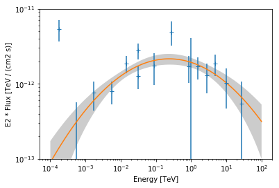
LogParabola

Parameters:

           name     value   error      unit      min max frozen
        --------- --------- ----- -------------- --- --- ------
        amplitude 1.930e-12   nan cm-2 s-1 TeV-1 nan nan  False
        reference 1.000e+00   nan            TeV nan nan   True
            alpha 2.151e+00   nan                nan nan  False
             beta 5.259e-02   nan                nan nan  False

[18]:

ax = flux_points.plot(energy_power=2)
log_parabola.plot(energy_range=[1e-4, 1e2] * u.TeV, ax=ax, energy_power=2)

# assign covariance for plotting
log_parabola.parameters.covariance = result_log_parabola.parameters.covariance

log_parabola.plot_error(
    energy_range=[1e-4, 1e2] * u.TeV, ax=ax, energy_power=2
)
ax.set_ylim(1e-13, 1e-11);

../_images/notebooks_sed_fitting_gammacat_fermi_32_0.png

Exercises¶

Fit a PowerLaw2 and ExponentialCutoffPowerLaw3FGL to the same data.
Fit a ExponentialCutoffPowerLaw model to Vela X (‘HESS J0835-455’) only and check if the best fit values correspond to the values given in the Gammacat catalog

What next?¶

This was an introduction to SED fitting in Gammapy.

If you would like to learn how to perform a full Poisson maximum likelihood spectral fit, please check out the spectrum analysis tutorial.
To learn more about other parts of Gammapy (e.g. Fermi-LAT and TeV data analysis), check out the other tutorial notebooks.
To see what’s available in Gammapy, browse the Gammapy docs or use the full-text search.
If you have any questions, ask on the mailing list .

[19]: