This is a fixed-text formatted version of a Jupyter notebook
- Try online

- You can contribute with your own notebooks in this GitHub repository.
- Source files: spectrum_simulation.ipynb | spectrum_simulation.py
Spectrum simulation for CTA
A quick example how to use the functions and classes in gammapy.spectrum in order to simulate and fit spectra.
We will simulate observations for the Cherenkov Telescope Array (CTA) first using a power law model without any background. Than we will add a power law shaped background component. The next part of the tutorial shows how to use user defined models for simulations and fitting.
We will use the following classes:
- gammapy.spectrum.SpectrumDatasetOnOff
- gammapy.spectrum.SpectrumSimulation
- gammapy.irf.load_cta_irfs
- gammapy.spectrum.models.PowerLaw
Setup
Same procedure as in every script …
[1]:
%matplotlib inline
import matplotlib.pyplot as plt
[2]:
import numpy as np
import astropy.units as u
from gammapy.spectrum import SpectrumSimulation
from gammapy.utils.fitting import Fit, Parameter
from gammapy.spectrum.models import PowerLaw
from gammapy.spectrum import models
from gammapy.irf import load_cta_irfs
Simulation of a single spectrum
To do a simulation, we need to define the observational parameters like the livetime, the offset, the energy range to perform the simulation for and the choice of spectral model. This will then be convolved with the IRFs, and Poission fluctuated, to get the simulated counts for each observation.
[3]:
# Define simulation parameters parameters
livetime = 1 * u.h
offset = 0.5 * u.deg
# Energy from 0.1 to 100 TeV with 10 bins/decade
energy = np.logspace(-1, 2, 31) * u.TeV
[4]:
# Define spectral model - a simple Power Law in this case
model_ref = PowerLaw(
    index=3.0,
    amplitude=2.5e-12 * u.Unit("cm-2 s-1 TeV-1"),
    reference=1 * u.TeV,
)
print(model_ref)
PowerLaw

Parameters:

           name     value   error      unit      min max frozen
        --------- --------- ----- -------------- --- --- ------
            index 3.000e+00   nan                nan nan  False
        amplitude 2.500e-12   nan cm-2 s-1 TeV-1 nan nan  False
        reference 1.000e+00   nan            TeV nan nan   True
Get and set the model parameters after initialising
The model parameters are stored in the Parameters object on the spectal model. Each model parameter is a Parameter instance. It has a value and a unit attribute, as well as a quantity property for convenience.
[5]:
print(model_ref.parameters)
Parameters
Parameter(name='index', value=3.0, factor=3.0, scale=1.0, unit='', min=nan, max=nan, frozen=False)
Parameter(name='amplitude', value=2.5e-12, factor=2.5e-12, scale=1.0, unit='cm-2 s-1 TeV-1', min=nan, max=nan, frozen=False)
Parameter(name='reference', value=1.0, factor=1.0, scale=1.0, unit='TeV', min=nan, max=nan, frozen=True)

covariance:
None
[6]:
print(model_ref.parameters["index"])
model_ref.parameters["index"].value = 2.1
print(model_ref.parameters["index"])
Parameter(name='index', value=3.0, factor=3.0, scale=1.0, unit='', min=nan, max=nan, frozen=False)
Parameter(name='index', value=2.1, factor=2.1, scale=1.0, unit='', min=nan, max=nan, frozen=False)
[7]:
# Load IRFs
filename = (
    "$GAMMAPY_DATA/cta-1dc/caldb/data/cta/1dc/bcf/South_z20_50h/irf_file.fits"
)
cta_irf = load_cta_irfs(filename)
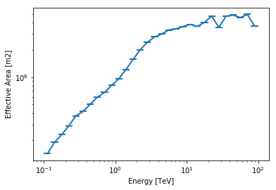
A quick look into the effective area and energy dispersion:
[8]:
aeff = cta_irf["aeff"].to_effective_area_table(offset=offset, energy=energy)
aeff.plot()
plt.loglog()
print(cta_irf["aeff"].data)
NDDataArray summary info
MapAxis

        name       : energy
        unit       : 'TeV'
        nbins      : 42
        node type  : edges
        edges min  : 1.3e-02 TeV
        edges max  : 2.0e+02 TeV
        interp     : log
MapAxis

        name       : offset
        unit       : 'deg'
        nbins      : 6
        node type  : edges
        edges min  : 0.0e+00 deg
        edges max  : 6.0e+00 deg
        interp     : lin
Data           : size =   252, min =  0.000 m2, max = 5371581.000 m2
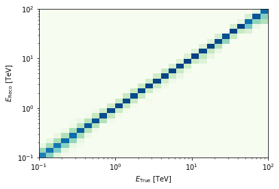
[9]:
edisp = cta_irf["edisp"].to_energy_dispersion(
    offset=offset, e_true=energy, e_reco=energy
)
edisp.plot_matrix()
print(edisp.data)
NDDataArray summary info
MapAxis

        name       : e_true
        unit       : 'TeV'
        nbins      : 30
        node type  : edges
        edges min  : 1.0e-01 TeV
        edges max  : 1.0e+02 TeV
        interp     : log
MapAxis

        name       : e_reco
        unit       : 'TeV'
        nbins      : 30
        node type  : edges
        edges min  : 1.0e-01 TeV
        edges max  : 1.0e+02 TeV
        interp     : log
Data           : size =   900, min =  0.000, max =  0.926
The SpectrumSimulation class does the work of convolving the model with the effective area and the energy dispersion, and then Poission fluctuating the counts. An obs_id is needed by SpectrumSimulation.simulate_obs() to keep track of the simulated spectra. Here, we just pass a dummy index, but while simulating observations in a loop, this needs to be updated.
[10]:
# Simulate data
sim = SpectrumSimulation(
    aeff=aeff, edisp=edisp, source_model=model_ref, livetime=livetime
)
sim.simulate_obs(seed=42, obs_id=0)
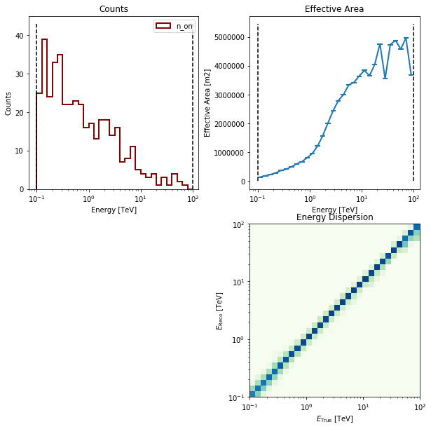
[11]:
# Take a quick look at the simulated counts
sim.obs.peek()
print(sim.obs)
<gammapy.spectrum.dataset.SpectrumDatasetOnOff object at 0x1c22485438>
Include Background
In this section we will include a background component. Furthermore, we will also simulate more than one observation and fit each one individually in order to get average fit results.
[12]:
# We assume a PowerLaw shape of the background as well
bkg_model = PowerLaw(
    index=2.5, amplitude=1e-11 * u.Unit("cm-2 s-1 TeV-1"), reference=1 * u.TeV
)
[13]:
%%time
# Now simulate 30 indepenent spectra using the same set of observation conditions.
n_obs = 30
seeds = np.arange(n_obs)

sim = SpectrumSimulation(
    aeff=aeff,
    edisp=edisp,
    source_model=model_ref,
    livetime=livetime,
    background_model=bkg_model,
    alpha=0.2,
)

sim.run(seeds)
print(sim.result)
print(sim.result[0])
[<gammapy.spectrum.dataset.SpectrumDatasetOnOff object at 0x1c222e8780>, <gammapy.spectrum.dataset.SpectrumDatasetOnOff object at 0x1c222e81d0>, <gammapy.spectrum.dataset.SpectrumDatasetOnOff object at 0x1c222e8d30>, <gammapy.spectrum.dataset.SpectrumDatasetOnOff object at 0x1c223fab38>, <gammapy.spectrum.dataset.SpectrumDatasetOnOff object at 0x1c223fac18>, <gammapy.spectrum.dataset.SpectrumDatasetOnOff object at 0x1c223faba8>, <gammapy.spectrum.dataset.SpectrumDatasetOnOff object at 0x1c223fa470>, <gammapy.spectrum.dataset.SpectrumDatasetOnOff object at 0x1c222e84e0>, <gammapy.spectrum.dataset.SpectrumDatasetOnOff object at 0x1c2240a940>, <gammapy.spectrum.dataset.SpectrumDatasetOnOff object at 0x1c2240a8d0>, <gammapy.spectrum.dataset.SpectrumDatasetOnOff object at 0x1c2240a358>, <gammapy.spectrum.dataset.SpectrumDatasetOnOff object at 0x1c22569b00>, <gammapy.spectrum.dataset.SpectrumDatasetOnOff object at 0x1c225695f8>, <gammapy.spectrum.dataset.SpectrumDatasetOnOff object at 0x1c22491e48>, <gammapy.spectrum.dataset.SpectrumDatasetOnOff object at 0x1c224914a8>, <gammapy.spectrum.dataset.SpectrumDatasetOnOff object at 0x1c22569908>, <gammapy.spectrum.dataset.SpectrumDatasetOnOff object at 0x1c222e8b70>, <gammapy.spectrum.dataset.SpectrumDatasetOnOff object at 0x1c224205f8>, <gammapy.spectrum.dataset.SpectrumDatasetOnOff object at 0x1c224206d8>, <gammapy.spectrum.dataset.SpectrumDatasetOnOff object at 0x1c22450198>, <gammapy.spectrum.dataset.SpectrumDatasetOnOff object at 0x1c22450518>, <gammapy.spectrum.dataset.SpectrumDatasetOnOff object at 0x1c22450908>, <gammapy.spectrum.dataset.SpectrumDatasetOnOff object at 0x1c22350908>, <gammapy.spectrum.dataset.SpectrumDatasetOnOff object at 0x1c22450c18>, <gammapy.spectrum.dataset.SpectrumDatasetOnOff object at 0x1c2240a6d8>, <gammapy.spectrum.dataset.SpectrumDatasetOnOff object at 0x1c22569f28>, <gammapy.spectrum.dataset.SpectrumDatasetOnOff object at 0x1c22350fd0>, <gammapy.spectrum.dataset.SpectrumDatasetOnOff object at 0x1c2246f048>, <gammapy.spectrum.dataset.SpectrumDatasetOnOff object at 0x1c2246fe80>, <gammapy.spectrum.dataset.SpectrumDatasetOnOff object at 0x1c2246f5c0>]
<gammapy.spectrum.dataset.SpectrumDatasetOnOff object at 0x1c222e8780>
CPU times: user 124 ms, sys: 2.71 ms, total: 126 ms
Wall time: 125 ms
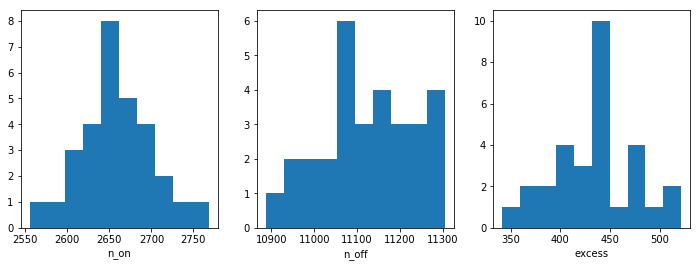
Before moving on to the fit let’s have a look at the simulated observations.
[14]:
n_on = [obs.total_stats.n_on for obs in sim.result]
n_off = [obs.total_stats.n_off for obs in sim.result]
excess = [obs.total_stats.excess for obs in sim.result]

fix, axes = plt.subplots(1, 3, figsize=(12, 4))
axes[0].hist(n_on)
axes[0].set_xlabel("n_on")
axes[1].hist(n_off)
axes[1].set_xlabel("n_off")
axes[2].hist(excess)
axes[2].set_xlabel("excess");
Now, we fit each simulated spectrum individually
[15]:
%%time
results = []
for obs in sim.result:
    dataset = obs
    dataset.model = model_ref.copy()
    fit = Fit([dataset])
    result = fit.optimize()
    results.append(
        {
            "index": result.parameters["index"].value,
            "amplitude": result.parameters["amplitude"].value,
        }
    )
CPU times: user 2.12 s, sys: 26 ms, total: 2.15 s
Wall time: 2.22 s
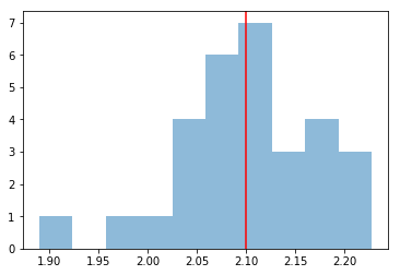
We take a look at the distribution of the fitted indices. This matches very well with the spectrum that we initially injected, index=2.1
[16]:
index = np.array([_["index"] for _ in results])
plt.hist(index, bins=10, alpha=0.5)
plt.axvline(x=model_ref.parameters["index"].value, color="red")
print("spectral index: {:.2f} +/- {:.2f}".format(index.mean(), index.std()))
spectral index: 2.10 +/- 0.07
Adding a user defined model
Many spectral models in gammapy are subclasses of SpectralModel. The list of available models is shown below.
[17]:
models.SpectralModel.__subclasses__()
[17]:
[gammapy.spectrum.models.ConstantModel,
 gammapy.spectrum.models.CompoundSpectralModel,
 gammapy.spectrum.models.PowerLaw,
 gammapy.spectrum.models.PowerLaw2,
 gammapy.spectrum.models.ExponentialCutoffPowerLaw,
 gammapy.spectrum.models.ExponentialCutoffPowerLaw3FGL,
 gammapy.spectrum.models.PLSuperExpCutoff3FGL,
 gammapy.spectrum.models.LogParabola,
 gammapy.spectrum.models.TableModel,
 gammapy.spectrum.models.ScaleModel,
 gammapy.spectrum.models.AbsorbedSpectralModel,
 gammapy.spectrum.models.NaimaModel,
 gammapy.spectrum.crab.MeyerCrabModel]
This section shows how to add a user defined spectral model.
To do that you need to subclass SpectralModel. All SpectralModel subclasses need to have an __init__ function, which sets up the Parameters of the model and a static function called evaluate where the mathematical expression for the model is defined.
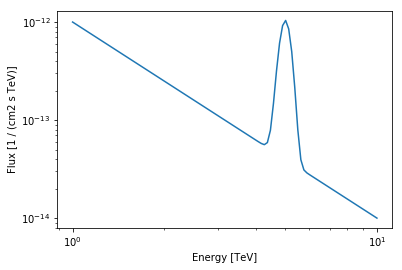
As an example we will use a PowerLaw plus a Gaussian (with fixed width).
[18]:
class UserModel(models.SpectralModel):
    def __init__(self, index, amplitude, reference, mean, width):
        super().__init__(
            [
                Parameter("index", index, min=0),
                Parameter("amplitude", amplitude, min=0),
                Parameter("reference", reference, frozen=True),
                Parameter("mean", mean, min=0),
                Parameter("width", width, min=0, frozen=True),
            ]
        )

    @staticmethod
    def evaluate(energy, index, amplitude, reference, mean, width):
        pwl = models.PowerLaw.evaluate(
            energy=energy,
            index=index,
            amplitude=amplitude,
            reference=reference,
        )
        gauss = amplitude * np.exp(-(energy - mean) ** 2 / (2 * width ** 2))
        return pwl + gauss
[19]:
model = UserModel(
    index=2,
    amplitude=1e-12 * u.Unit("cm-2 s-1 TeV-1"),
    reference=1 * u.TeV,
    mean=5 * u.TeV,
    width=0.2 * u.TeV,
)
print(model)
UserModel

Parameters:

           name     value   error      unit         min    max frozen
        --------- --------- ----- -------------- --------- --- ------
            index 2.000e+00   nan                0.000e+00 nan  False
        amplitude 1.000e-12   nan cm-2 s-1 TeV-1 0.000e+00 nan  False
        reference 1.000e+00   nan            TeV       nan nan   True
             mean 5.000e+00   nan            TeV 0.000e+00 nan  False
            width 2.000e-01   nan            TeV 0.000e+00 nan   True
[20]:
energy_range = [1, 10] * u.TeV
model.plot(energy_range=energy_range);
Exercises
- Change the observation time to something longer or shorter. Does the observation and spectrum results change as you expected?
- Change the spectral model, e.g. add a cutoff at 5 TeV, or put a steep-spectrum source with spectral index of 4.0
- Simulate spectra with the spectral model we just defined. How much observation duration do you need to get back the injected parameters?
What next?
In this tutorial we simulated and analysed the spectrum of source using CTA prod 2 IRFs.
If you’d like to go further, please see the other tutorial notebooks.