This is a fixed-text formatted version of a Jupyter notebook
- Try online

- You can contribute with your own notebooks in this GitHub repository.
- Source files: simulate_3d.ipynb | simulate_3d.py
3D simulation and fitting
This tutorial shows how to do a 3D map-based simulation and fit.
For a tutorial on how to do a 3D map analyse of existing data, see the analysis_3d tutorial.
This can be useful to do a performance / sensitivity study, or to evaluate the capabilities of Gammapy or a given analysis method. Note that is is a binned simulation as is e.g. done also in Sherpa for Chandra, not an event sampling and anbinned analysis as is done e.g. in the Fermi ST or ctools.
Imports and versions
[1]:
%matplotlib inline
import matplotlib.pyplot as plt
[2]:
import numpy as np
import astropy.units as u
from astropy.coordinates import Angle
from gammapy.irf import load_cta_irfs
from gammapy.maps import WcsGeom, MapAxis, WcsNDMap
from gammapy.spectrum.models import PowerLaw
from gammapy.image.models import SkyGaussian
from gammapy.cube.models import SkyModel, BackgroundModel
from gammapy.cube import MapDataset, PSFKernel
from gammapy.cube import make_map_exposure_true_energy, make_map_background_irf
from gammapy.utils.fitting import Fit
from gammapy.data import FixedPointingInfo
[3]:
!gammapy info --no-envvar --no-dependencies --no-system
Gammapy package:

        path                   : /Users/adonath/github/adonath/gammapy/gammapy
        version                : 0.12
Simulate
[4]:
filename = (
    "$GAMMAPY_DATA/cta-1dc/caldb/data/cta/1dc/bcf/South_z20_50h/irf_file.fits"
)
irfs = load_cta_irfs(filename)
[5]:
# Define sky model to simulate the data
spatial_model = SkyGaussian(lon_0="0.2 deg", lat_0="0.1 deg", sigma="0.3 deg")
spectral_model = PowerLaw(
    index=3, amplitude="1e-11 cm-2 s-1 TeV-1", reference="1 TeV"
)
sky_model = SkyModel(
    spatial_model=spatial_model, spectral_model=spectral_model
)
print(sky_model)
SkyModel

Parameters:

           name     value   error      unit         min        max    frozen
        --------- --------- ----- -------------- ---------- --------- ------
            lon_0 2.000e-01   nan            deg -1.800e+02 1.800e+02  False
            lat_0 1.000e-01   nan            deg -9.000e+01 9.000e+01  False
            sigma 3.000e-01   nan            deg  0.000e+00       nan  False
            index 3.000e+00   nan                       nan       nan  False
        amplitude 1.000e-11   nan cm-2 s-1 TeV-1        nan       nan  False
        reference 1.000e+00   nan            TeV        nan       nan   True
[6]:
# Define map geometry
axis = MapAxis.from_edges(
    np.logspace(-1.0, 1.0, 10), unit="TeV", name="energy", interp="log"
)
geom = WcsGeom.create(
    skydir=(0, 0), binsz=0.02, width=(5, 4), coordsys="GAL", axes=[axis]
)
[7]:
# Define some observation parameters
# We read in the pointing info from one of the 1dc event list files as an example
pointing = FixedPointingInfo.read(
    "$GAMMAPY_DATA/cta-1dc/data/baseline/gps/gps_baseline_110380.fits"
)

livetime = 1 * u.hour
offset_max = 2 * u.deg
offset = Angle("2 deg")
[8]:
exposure = make_map_exposure_true_energy(
pointing=pointing.radec, livetime=livetime, aeff=irfs["aeff"], geom=geom
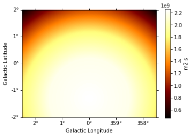
)
exposure.slice_by_idx({"energy": 3}).plot(add_cbar=True);
[9]:
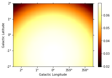
background = make_map_background_irf(
    pointing=pointing, ontime=livetime, bkg=irfs["bkg"], geom=geom
)
background.slice_by_idx({"energy": 3}).plot(add_cbar=True);
WARNING: Tried to get polar motions for times after IERS data is valid. Defaulting to polar motion from the 50-yr mean for those. This may affect precision at the 10s of arcsec level [astropy.coordinates.builtin_frames.utils]
[10]:
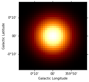
psf = irfs["psf"].to_energy_dependent_table_psf(theta=offset)
psf_kernel = PSFKernel.from_table_psf(psf, geom, max_radius=0.3 * u.deg)
psf_kernel.psf_kernel_map.sum_over_axes().plot(stretch="log");
[11]:
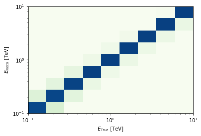
energy = axis.edges
edisp = irfs["edisp"].to_energy_dispersion(
    offset, e_reco=energy, e_true=energy
)
edisp.plot_matrix();
Now we have to compute npred maps, i.e. “predicted counts per pixel” given the model and the observation infos: exposure, background, PSF and EDISP. For this we use the MapDataset object:
[12]:
background_model = BackgroundModel(background)
dataset = MapDataset(
    model=sky_model,
    exposure=exposure,
    background_model=background_model,
    psf=psf_kernel,
    edisp=edisp,
)
[13]:
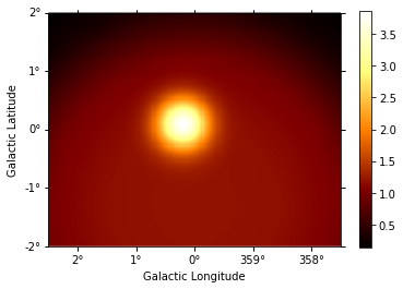
npred = dataset.npred()
[14]:
npred.sum_over_axes().plot(add_cbar=True);
[15]:
# This one line is the core of how to simulate data when
# using binned simulation / analysis: you Poisson fluctuate
# npred to obtain simulated observed counts.
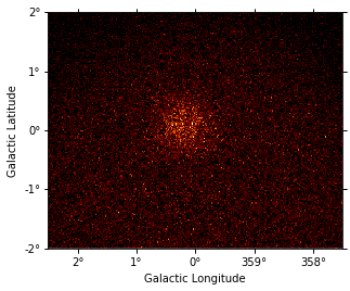
# Compute counts as a Poisson fluctuation
rng = np.random.RandomState(seed=42)
counts = rng.poisson(npred.data)
counts_map = WcsNDMap(geom, counts)
[16]:
counts_map.sum_over_axes().plot();
Fit
Now let’s analyse the simulated data. Here we just fit it again with the same model we had before, but you could do any analysis you like here, e.g. fit a different model, or do a region-based analysis, …
[17]:
# Define sky model to fit the data
spatial_model = SkyGaussian(lon_0="0.1 deg", lat_0="0.1 deg", sigma="0.5 deg")
spectral_model = PowerLaw(
    index=2, amplitude="1e-11 cm-2 s-1 TeV-1", reference="1 TeV"
)
model = SkyModel(spatial_model=spatial_model, spectral_model=spectral_model)
print(model)
SkyModel

Parameters:

           name     value   error      unit         min        max    frozen
        --------- --------- ----- -------------- ---------- --------- ------
            lon_0 1.000e-01   nan            deg -1.800e+02 1.800e+02  False
            lat_0 1.000e-01   nan            deg -9.000e+01 9.000e+01  False
            sigma 5.000e-01   nan            deg  0.000e+00       nan  False
            index 2.000e+00   nan                       nan       nan  False
        amplitude 1.000e-11   nan cm-2 s-1 TeV-1        nan       nan  False
        reference 1.000e+00   nan            TeV        nan       nan   True
[18]:
# We do not want to fit the background in this case, so we will freeze the parameters
background_model.parameters["norm"].value = 1.0
background_model.parameters["norm"].frozen = True
background_model.parameters["tilt"].frozen = True

print(background_model)
BackgroundModel

Parameters:

           name     value   error unit    min    max frozen
        --------- --------- ----- ---- --------- --- ------
             norm 1.000e+00   nan      0.000e+00 nan   True
             tilt 0.000e+00   nan            nan nan   True
        reference 1.000e+00   nan  TeV       nan nan   True
[19]:
dataset = MapDataset(
    model=model,
    exposure=exposure,
    counts=counts_map,
    background_model=background_model,
    psf=psf_kernel,
    edisp=edisp,
)
[20]:
%%time
fit = Fit(dataset)
result = fit.run(optimize_opts={"print_level": 1})
| FCN = 233997.8495429449 | TOTAL NCALL = 214 | NCALLS = 214 |
| EDM = 5.36146884348607e-06 | GOAL EDM = 1e-05 | UP = 1.0 |
| Valid | Valid Param | Accurate Covar | PosDef | Made PosDef |
| True | True | True | True | False |
| Hesse Fail | HasCov | Above EDM | Reach calllim | |
| False | True | False | False |
| + | Name | Value | Hesse Error | Minos Error- | Minos Error+ | Limit- | Limit+ | Fixed? |
| 0 | par_000_lon_0 | 18.5861 | 0.881872 | -18000 | 18000 | No | ||
| 1 | par_001_lat_0 | 0.876831 | 0.0874743 | -900 | 900 | No | ||
| 2 | par_002_sigma | 2.96346 | 0.0609922 | 0 | No | |||
| 3 | par_003_index | 3.05558 | 0.0305726 | No | ||||
| 4 | par_004_amplitude | 0.905969 | 0.0461428 | No |
CPU times: user 15.4 s, sys: 331 ms, total: 15.7 s
Wall time: 7.89 s
True model:
[21]:
print(sky_model)
SkyModel

Parameters:

           name     value   error      unit         min        max    frozen
        --------- --------- ----- -------------- ---------- --------- ------
            lon_0 2.000e-01   nan            deg -1.800e+02 1.800e+02  False
            lat_0 1.000e-01   nan            deg -9.000e+01 9.000e+01  False
            sigma 3.000e-01   nan            deg  0.000e+00       nan  False
            index 3.000e+00   nan                       nan       nan  False
        amplitude 1.000e-11   nan cm-2 s-1 TeV-1        nan       nan  False
        reference 1.000e+00   nan            TeV        nan       nan   True
Best-fit model:
[22]:
print(model)
SkyModel

Parameters:

           name     value   error      unit         min        max    frozen
        --------- --------- ----- -------------- ---------- --------- ------
            lon_0 1.859e-01   nan            deg -1.800e+02 1.800e+02  False
            lat_0 8.768e-02   nan            deg -9.000e+01 9.000e+01  False
            sigma 2.963e-01   nan            deg  0.000e+00       nan  False
            index 3.056e+00   nan                       nan       nan  False
        amplitude 9.060e-12   nan cm-2 s-1 TeV-1        nan       nan  False
        reference 1.000e+00   nan            TeV        nan       nan   True
To get the errors on the model, we can check the covariance table:
[23]:
result.parameters.covariance_to_table()
[23]:
| name | lon_0 | lat_0 | sigma | index | amplitude | reference | norm | tilt |
|---|---|---|---|---|---|---|---|---|
| str9 | float64 | float64 | float64 | float64 | float64 | float64 | float64 | float64 |
| lon_0 | 7.777e-05 | 3.525e-07 | -9.334e-08 | -4.088e-06 | 4.998e-17 | 0.000e+00 | 0.000e+00 | 0.000e+00 |
| lat_0 | 3.525e-07 | 7.652e-05 | 1.826e-06 | 3.123e-06 | 4.978e-17 | 0.000e+00 | 0.000e+00 | 0.000e+00 |
| sigma | -9.334e-08 | 1.826e-06 | 3.720e-05 | -5.988e-07 | 7.925e-16 | 0.000e+00 | 0.000e+00 | 0.000e+00 |
| index | -4.088e-06 | 3.123e-06 | -5.988e-07 | 9.347e-04 | -1.197e-14 | 0.000e+00 | 0.000e+00 | 0.000e+00 |
| amplitude | 4.998e-17 | 4.978e-17 | 7.925e-16 | -1.197e-14 | 2.129e-25 | 0.000e+00 | 0.000e+00 | 0.000e+00 |
| reference | 0.000e+00 | 0.000e+00 | 0.000e+00 | 0.000e+00 | 0.000e+00 | 0.000e+00 | 0.000e+00 | 0.000e+00 |
| norm | 0.000e+00 | 0.000e+00 | 0.000e+00 | 0.000e+00 | 0.000e+00 | 0.000e+00 | 0.000e+00 | 0.000e+00 |
| tilt | 0.000e+00 | 0.000e+00 | 0.000e+00 | 0.000e+00 | 0.000e+00 | 0.000e+00 | 0.000e+00 | 0.000e+00 |
| reference | 0.000e+00 | 0.000e+00 | 0.000e+00 | 0.000e+00 | 0.000e+00 | 0.000e+00 | 0.000e+00 | 0.000e+00 |
[24]:
# Or, to see the value of and error on an individual parameter, say index:
print(result.parameters["index"].value, result.parameters.error("index"))
3.0555770550063204 0.03057263305196295
[25]:
# TODO: show e.g. how to make a residual image