This is a fixed-text formatted version of a Jupyter notebook
- Try online

- You can contribute with your own notebooks in this GitHub repository.
- Source files: light_curve.ipynb | light_curve.py
Light curves
Introduction
This tutorial explain how to compute a light curve with Gammapy.
We will use the four Crab nebula observations from the H.E.S.S. first public test data release and compute per-observation fluxes. The Crab nebula is not known to be variable at TeV energies, so we expect constant brightness within statistical and systematic errors.
The main classes we will use are:
Setup
As usual, we’ll start with some setup…
[1]:
%matplotlib inline
import matplotlib.pyplot as plt
import astropy.units as u
from astropy.coordinates import SkyCoord, Angle
from regions import CircleSkyRegion
from gammapy.utils.energy import EnergyBounds
from gammapy.data import DataStore
from gammapy.spectrum import SpectrumExtraction
from gammapy.spectrum.models import PowerLaw
from gammapy.background import ReflectedRegionsBackgroundEstimator
from gammapy.time import LightCurveEstimator
Spectrum
The LightCurveEstimator is based on a 1d spectral analysis within each time bin. So before we can make the light curve, we have to extract 1d spectra.
[2]:
data_store = DataStore.from_dir("$GAMMAPY_DATA/hess-dl3-dr1/")
[3]:
mask = data_store.obs_table["TARGET_NAME"] == "Crab"
obs_ids = data_store.obs_table["OBS_ID"][mask].data
observations = data_store.get_observations(obs_ids)
print(observations)
Observations
Number of observations: 4
Info for OBS_ID = 23523
- Start time: 53343.92
- Pointing pos: RA 83.63 deg / Dec 21.51 deg
- Observation duration: 1687.0 s
- Dead-time fraction: 6.240 %
Info for OBS_ID = 23526
- Start time: 53343.95
- Pointing pos: RA 83.63 deg / Dec 22.51 deg
- Observation duration: 1683.0 s
- Dead-time fraction: 6.555 %
Info for OBS_ID = 23559
- Start time: 53345.96
- Pointing pos: RA 85.25 deg / Dec 22.01 deg
- Observation duration: 1686.0 s
- Dead-time fraction: 6.398 %
Info for OBS_ID = 23592
- Start time: 53347.91
- Pointing pos: RA 82.01 deg / Dec 22.01 deg
- Observation duration: 1686.0 s
- Dead-time fraction: 6.212 %
[4]:
# Target definition
target_position = SkyCoord(ra=83.63308, dec=22.01450, unit="deg")
on_region_radius = Angle("0.2 deg")
on_region = CircleSkyRegion(center=target_position, radius=on_region_radius)
[5]:
%%time
bkg_estimator = ReflectedRegionsBackgroundEstimator(
    on_region=on_region, observations=observations
)
bkg_estimator.run()
CPU times: user 814 ms, sys: 16.1 ms, total: 830 ms
Wall time: 833 ms
[6]:
%%time
ebounds = EnergyBounds.equal_log_spacing(0.7, 100, 50, unit="TeV")
extraction = SpectrumExtraction(
    observations=observations,
    bkg_estimate=bkg_estimator.result,
    containment_correction=False,
    e_reco=ebounds,
    e_true=ebounds,
)
extraction.run()
spectrum_observations = extraction.spectrum_observations
CPU times: user 883 ms, sys: 24 ms, total: 907 ms
Wall time: 947 ms
Light curve estimation
OK, so now that we have prepared 1D spectra (not spectral models, just the 1D counts and exposure and 2D energy dispersion matrix), we can compute a lightcurve.
To compute the light curve, a spectral model shape has to be assumed, and an energy band chosen. The method is then to adjust the amplitude parameter of the spectral model in each time bin to the data, resulting in a flux measurement in each time bin.
[7]:
# Creat list of time bin intervals
# Here we do one time bin per observation
time_intervals = [(obs.tstart, obs.tstop) for obs in observations]
[8]:
# Assumed spectral model
spectral_model = PowerLaw(
    index=2, amplitude=2.0e-11 * u.Unit("1 / (cm2 s TeV)"), reference=1 * u.TeV
)
[9]:
energy_range = [1, 100] * u.TeV
[10]:
%%time
lc_estimator = LightCurveEstimator(extraction)
lc = lc_estimator.light_curve(
    time_intervals=time_intervals,
    spectral_model=spectral_model,
    energy_range=energy_range,
)
CPU times: user 1.05 s, sys: 29.2 ms, total: 1.08 s
Wall time: 1.57 s
Results
The light curve measurement result is stored in a table. Let’s have a look at the results:
[11]:
print(lc.table.colnames)
['time_min', 'time_max', 'flux', 'flux_err', 'flux_ul', 'is_ul', 'livetime', 'alpha', 'n_on', 'n_off', 'measured_excess', 'expected_excess']
[12]:
lc.table["time_min", "time_max", "flux", "flux_err"]
[12]:
| time_min | time_max | flux | flux_err |
|---|---|---|---|
| 1 / (cm2 s) | 1 / (cm2 s) | ||
| float64 | float64 | float64 | float64 |
| 53343.92234009259 | 53343.94186555556 | 1.8415530028767494e-11 | 1.901096920855279e-12 |
| 53343.95421509259 | 53343.97369425926 | 1.998670964314257e-11 | 2.0213838634857846e-12 |
| 53345.96198129629 | 53345.98149518518 | 2.193396904197396e-11 | 2.5543071221453397e-12 |
| 53347.913196574074 | 53347.93271046296 | 2.321856396079876e-11 | 2.5699816445058737e-12 |
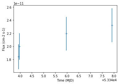
[13]:
lc.plot();
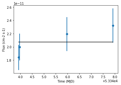
[14]:
# Let's compare to the expected flux of this source
from gammapy.spectrum import CrabSpectrum

crab_spec = CrabSpectrum().model
crab_flux = crab_spec.integral(*energy_range).to("cm-2 s-1")
crab_flux
[14]:
[15]:
ax = lc.plot(marker="o", lw=2)
ax.hlines(
    crab_flux.value,
    xmin=lc.table["time_min"].min(),
    xmax=lc.table["time_max"].max(),
);
Exercises
- Change the assumed spectral model shape (e.g. to a steeper power-law), and see how the integral flux estimate for the lightcurve changes.
- Try a time binning where you split the observation time for every run into two time bins.
- Try to analyse the PKS 2155 flare data from the H.E.S.S. first public test data release. Start with per-observation fluxes, and then try fluxes within 5 minute time bins for one or two of the observations where the source was very bright.
[16]: