This is a fixed-text formatted version of a Jupyter notebook.
- Try online

- You can contribute with your own notebooks in this GitHub repository.
- Source files: analysis_3d.ipynb | analysis_3d.py
3D analysis
This tutorial shows how to run a 3D map-based analysis using three example observations of the Galactic center region with CTA.
Setup
In [1]:
%matplotlib inline
import matplotlib.pyplot as plt
In [2]:
import numpy as np
import astropy.units as u
from astropy.coordinates import SkyCoord
from gammapy.extern.pathlib import Path
from gammapy.data import DataStore
from gammapy.irf import EnergyDispersion
from gammapy.maps import WcsGeom, MapAxis, Map
from gammapy.cube import MapMaker, PSFKernel, MapFit
from gammapy.cube.models import SkyModel
from gammapy.spectrum.models import PowerLaw
from gammapy.image.models import SkyGaussian, SkyPointSource
from regions import CircleSkyRegion
In [3]:
!gammapy info --no-envvar --no-dependencies --no-system
Gammapy package:

        path                   : /Users/jer/git/gammapy/gammapy
        version                : 0.8
Prepare modeling input data
Prepare input maps
We first use the DataStore object to access the CTA observations and
retrieve a list of observations by passing the observations IDs to the
.obs_list() method:
In [4]:
# Define which data to use
data_store = DataStore.from_dir("$GAMMAPY_DATA/cta-1dc/index/gps/")
obs_ids = [110380, 111140, 111159]
obs_list = data_store.obs_list(obs_ids)
Now we define a reference geometry for our analysis, We choose a WCS based gemoetry with a binsize of 0.02 deg and also define an energy axis:
In [5]:
energy_axis = MapAxis.from_edges(
    np.logspace(-1., 1., 10), unit="TeV", name="energy", interp="log"
)
geom = WcsGeom.create(
    skydir=(0, 0),
    binsz=0.02,
    width=(10, 8),
    coordsys="GAL",
    proj="CAR",
    axes=[energy_axis],
)
The MapMaker object is initialized with this reference geometry and
a field of view cut of 4 deg:
In [6]:
%%time
maker = MapMaker(geom, offset_max=4. * u.deg)
maps = maker.run(obs_list)
CPU times: user 12.8 s, sys: 2.66 s, total: 15.5 s
Wall time: 15.5 s
The maps are prepare by calling the .run() method and passing the
observation list obs_list. The .run() method returns a Python
dict containing a counts, background and exposure map:
In [7]:
print(maps)
{'counts': WcsNDMap

        geom  : WcsGeom
        axes  : lon, lat, energy
        shape : (500, 400, 9)
        ndim  : 3
        unit  : ''
        dtype : float32
, 'exposure': WcsNDMap

        geom  : WcsGeom
        axes  : lon, lat, energy
        shape : (500, 400, 9)
        ndim  : 3
        unit  : 'm2 s'
        dtype : float32
, 'background': WcsNDMap

        geom  : WcsGeom
        axes  : lon, lat, energy
        shape : (500, 400, 9)
        ndim  : 3
        unit  : ''
        dtype : float32
}
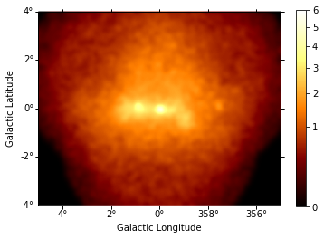
This is what the summed counts image looks like:
In [8]:
counts = maps["counts"].sum_over_axes()
counts.smooth(width=0.1 * u.deg).plot(stretch="sqrt", add_cbar=True, vmax=6);
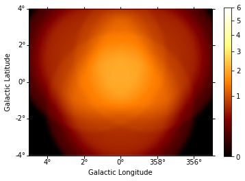
And the background image:
In [9]:
background = maps["background"].sum_over_axes()
background.smooth(width=0.1 * u.deg).plot(
    stretch="sqrt", add_cbar=True, vmax=6
);
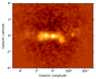
We can also compute an excess image just with a few lines of code:
In [10]:
excess = Map.from_geom(geom.to_image())
excess.data = counts.data - background.data
excess.smooth(5).plot(stretch="sqrt");
Prepare IRFs
To estimate the mean PSF across all observations at a given source
position src_pos, we use the obs_list.make_mean_psf() method:
In [11]:
# mean PSF
src_pos = SkyCoord(0, 0, unit="deg", frame="galactic")
table_psf = obs_list.make_mean_psf(src_pos)

# PSF kernel used for the model convolution
psf_kernel = PSFKernel.from_table_psf(table_psf, geom, max_radius="0.3 deg")
To estimate the mean energy dispersion across all observations at a
given source position src_pos, we use the
obs_list.make_mean_edisp() method:
In [12]:
# define energy grid
energy = energy_axis.edges * energy_axis.unit

# mean edisp
edisp = obs_list.make_mean_edisp(
    position=src_pos, e_true=energy, e_reco=energy
)
Save maps and IRFs to disk
It is common to run the preparation step independent of the likelihood fit, because often the preparation of maps, PSF and energy dispersion is slow if you have a lot of data. We first create a folder:
In [13]:
path = Path("analysis_3d")
path.mkdir(exist_ok=True)
And the write the maps and IRFs to disk by calling the dedicated
.write() methods:
In [14]:
# write maps
maps["counts"].write(str(path / "counts.fits"), overwrite=True)
maps["background"].write(str(path / "background.fits"), overwrite=True)
maps["exposure"].write(str(path / "exposure.fits"), overwrite=True)

# write IRFs
psf_kernel.write(str(path / "psf.fits"), overwrite=True)
edisp.write(str(path / "edisp.fits"), overwrite=True)
Likelihood fit
Reading maps and IRFs
As first step we read in the maps and IRFs that we have saved to disk again:
In [15]:
# read maps
maps = {
    "counts": Map.read(str(path / "counts.fits")),
    "background": Map.read(str(path / "background.fits")),
    "exposure": Map.read(str(path / "exposure.fits")),
}

# read IRFs
psf_kernel = PSFKernel.read(str(path / "psf.fits"))
edisp = EnergyDispersion.read(str(path / "edisp.fits"))
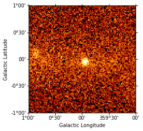
Let’s cut out only part of the maps, so that we the fitting step does not take so long:
In [16]:
cmaps = {
    name: m.cutout(SkyCoord(0, 0, unit="deg", frame="galactic"), 2 * u.deg)
    for name, m in maps.items()
}
cmaps["counts"].sum_over_axes().plot(stretch="sqrt");
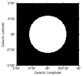
Fit mask
To select a certain spatial region and/or energy range for the fit we can create a fit mask:
In [17]:
mask = Map.from_geom(cmaps["counts"].geom)

region = CircleSkyRegion(center=src_pos, radius=0.6 * u.deg)
mask.data = mask.geom.region_mask([region])

mask.get_image_by_idx((0,)).plot();
In addition we also exclude the range below 0.3 TeV for the fit:
In [18]:
coords = mask.geom.get_coord()
mask.data &= coords["energy"] > 0.3
Model fit
No we are ready for the actual likelihood fit. We first define the model as a combination of a point source with a powerlaw:
In [19]:
spatial_model = SkyPointSource(lon_0="0.01 deg", lat_0="0.01 deg")
spectral_model = PowerLaw(
    index=2.2, amplitude="3e-12 cm-2 s-1 TeV-1", reference="1 TeV"
)
model = SkyModel(spatial_model=spatial_model, spectral_model=spectral_model)
Now we set up the MapFit object by passing the prepared maps, IRFs
as well as the model:
In [20]:
fit = MapFit(
    model=model,
    counts=cmaps["counts"],
    exposure=cmaps["exposure"],
    background=cmaps["background"],
    mask=mask,
    psf=psf_kernel,
    edisp=edisp,
)
No we run the model fit:
In [21]:
%%time
result = fit.run(optimize_opts={"print_level": 1})
| FCN = 14281.494006433117 | TOTAL NCALL = 162 | NCALLS = 162 |
| EDM = 7.25507095654257e-05 | GOAL EDM = 1e-05 | UP = 1.0 |
| Valid | Valid Param | Accurate Covar | PosDef | Made PosDef |
| True | True | True | True | False |
| Hesse Fail | HasCov | Above EDM | Reach calllim | |
| False | True | False | False |
| + | Name | Value | Hesse Error | Minos Error- | Minos Error+ | Limit- | Limit+ | Fixed? |
| 0 | par_000_lon_0 | -4.82863 | 0.219172 | No | ||||
| 1 | par_001_lat_0 | -5.2709 | 0.217971 | No | ||||
| 2 | par_002_index | 2.37661 | 0.0602493 | No | ||||
| 3 | par_003_amplitude | 0.27121 | 0.0149849 | No | ||||
| 4 | par_004_reference | 1 | 1 | 0 | Yes |
CPU times: user 3.36 s, sys: 58.1 ms, total: 3.42 s
Wall time: 3.42 s
Check model fit
Finally we check the model fit by cmputing a residual image. For this we first get the number of predicted counts from the fit evaluator:
In [22]:
npred = fit.evaluator.compute_npred()
And compute a residual image:
In [23]:
residual = Map.from_geom(cmaps["counts"].geom)
residual.data = cmaps["counts"].data - npred.data
In [24]:
residual.sum_over_axes().smooth(width=0.05 * u.deg).plot(
    cmap="coolwarm", vmin=-3, vmax=3, add_cbar=True
);
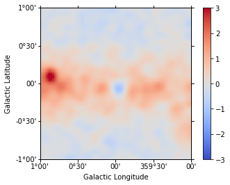
Apparently our model should be improved by adding a component for diffuse Galactic emission and at least one second point source (see exercises at the end of the notebook).
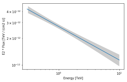
We can also plot the best fit spectrum:
In [25]:
spec = result.model.spectral_model
energy_range = [0.3, 10] * u.TeV
spec.plot(energy_range=energy_range, energy_power=2)
ax = spec.plot_error(energy_range=energy_range, energy_power=2)
Exercises
- Analyse the second source in the field of view: G0.9+0.1
- Run the model fit with energy dispersion (pass edisp to MapFit)