This is a fixed-text formatted version of a Jupyter notebook.
- Try online

- You can contribute with your own notebooks in this GitHub repository.
- Source files: first_steps.ipynb | first_steps.py
Getting started with Gammapy
Introduction
This is a getting started tutorial for Gammapy.
In this tutorial we will use the Second Fermi-LAT Catalog of High-Energy Sources (2FHL) catalog, corresponding event list and images to learn how to work with some of the central Gammapy data structures.
We will cover the following topics:
- Sky maps
- We will learn how to handle image based data with gammapy using a Fermi-LAT 2FHL example image. We will work with the following classes:
- Event lists
- We will learn how to handle event lists with Gammapy. Important for this are the following classes:
- Source catalogs
- We will show how to load source catalogs with Gammapy and explore the data using the following classes:
- Spectral models and flux points
- We will pick an example source and show how to plot its spectral
model and flux points. For this we will use the following classes:
- gammapy.spectrum.SpectralModel, specifically the PowerLaw2 model.
- gammapy.spectrum.FluxPoints
- astropy.table.Table
- We will pick an example source and show how to plot its spectral
model and flux points. For this we will use the following classes:
If you’re not yet familiar with the listed Astropy classes, maybe check out the Astropy introduction for Gammapy users first.
Setup
Important: to run this tutorial the environment variable
GAMMAPY_EXTRA must be defined and point to the directory, where the
gammapy-extra is respository located on your machine. To check whether
your setup is correct you can execute the following cell:
In [1]:
import os

path = os.path.expandvars("$GAMMAPY_DATA")

if not os.path.exists(path):
    raise Exception("gammapy-data repository not found!")
else:
    print("Great your setup is correct!")
Great your setup is correct!
In case you encounter an error, you can un-comment and execute the following cell to continue. But we recommend to set up your enviroment correctly as decribed here after you are done with this notebook.
In [2]:
# os.environ['GAMMAPY_DATA'] = os.path.join(os.getcwd(), '..')
Now we can continue with the usual IPython notebooks and Python imports:
In [3]:
%matplotlib inline
import matplotlib.pyplot as plt
In [4]:
import numpy as np
import astropy.units as u
from astropy.coordinates import SkyCoord
from astropy.visualization import simple_norm
Maps
The gammapy.maps package contains classes to work with sky images and cubes.
In this section, we will use a simple 2D sky image and will learn how to:
- Read sky images from FITS files
- Smooth images
- Plot images
- Cutout parts from images
- Reproject images to different WCS
In [5]:
from gammapy.maps import Map

vela_2fhl = Map.read(
    "$GAMMAPY_DATA/fermi_2fhl/fermi_2fhl_vela.fits.gz", hdu="COUNTS"
)
As the FITS file fermi_2fhl_vela.fits.gz contains mutiple image
extensions and a map can only represent a single image, we explicitely
specify to read the extension called ‘COUNTS’.
The image is a WCSNDMap object:
In [6]:
vela_2fhl
Out[6]:
WcsNDMap

    geom  : WcsGeom
    axes  : lon, lat
    shape : (320, 180)
    ndim  : 2
    unit  : ''
    dtype : >f8
The shape of the image is 320x180 pixel and it is defined using a cartesian projection in galactic coordinates.
The geom attribute is a WcsGeom object:
In [7]:
vela_2fhl.geom
Out[7]:
WcsGeom

    axes       : lon, lat
    shape      : (320, 180)
    ndim       : 2
    coordsys   : GAL
    projection : CAR
    center     : 266.0 deg, -1.2 deg
    width      : 32.0 x 18.0 deg
Let’s take a closer look a the .data attribute:
In [8]:
vela_2fhl.data
Out[8]:
array([[ 0.,  0.,  0., ...,  0.,  0.,  0.],
       [ 0.,  0.,  0., ...,  0.,  0.,  0.],
       [ 0.,  0.,  0., ...,  0.,  0.,  0.],
       ...,
       [ 0.,  0.,  0., ...,  0.,  0.,  0.],
       [ 0.,  0.,  0., ...,  0.,  0.,  0.],
       [ 0.,  0.,  0., ...,  0.,  0.,  0.]])
That looks familiar! It just an ordinary 2 dimensional numpy array, which means you can apply any known numpy method to it:
In [9]:
print(
    "Total number of counts in the image: {:.0f}".format(vela_2fhl.data.sum())
)
Total number of counts in the image: 1567
To show the image on the screen we can use the plot method. It
basically calls
plt.imshow,
passing the vela_2fhl.data attribute but in addition handles axis
with world coordinates using
wcsaxes and defines some
defaults for nicer plots (e.g. the colormap ‘afmhot’):
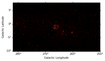
In [10]:
vela_2fhl.plot();
To make the structures in the image more visible we will smooth the data
using a Gausian kernel with a radius of 0.5 deg. Again smooth() is a
wrapper around existing functionality from the scientific Python
libraries. In this case it is Scipy’s
gaussian_filter
method. For convenience the kernel shape can be specified with as string
and the smoothing radius with a quantity. It returns again a map object,
that we can plot directly the same way we did above:
In [11]:
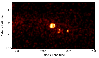
vela_2fhl_smoothed = vela_2fhl.smooth(kernel="gauss", width=0.2 * u.deg)
In [12]:
vela_2fhl_smoothed.plot();
The smoothed plot already looks much nicer, but still the image is
rather large. As we are mostly interested in the inner part of the
image, we will cut out a quadratic region of the size 9 deg x 9 deg
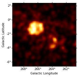
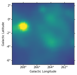
around Vela. Therefore we use Map.cutout to make a cutout map:
In [13]:
# define center and size of the cutout region
center = SkyCoord(265.0, -2.0, unit="deg", frame="galactic")
vela_2fhl_cutout = vela_2fhl_smoothed.cutout(center, 9 * u.deg)
vela_2fhl_cutout.plot();
To make this exercise a bit more scientifically useful, we will load a second image containing WMAP data from the same region:
In [14]:
vela_wmap = Map.read("$GAMMAPY_DATA/images/Vela_region_WMAP_K.fits")

# define a norm to stretch the data, so it is better visible
norm = simple_norm(vela_wmap.data, stretch="sqrt", max_percent=99.9)
vela_wmap.plot(cmap="viridis", norm=norm);
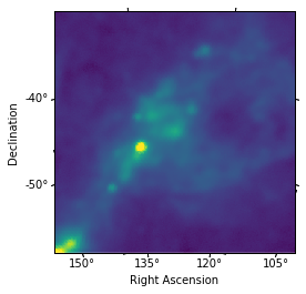
In order to make the structures in the data better visible we used the
simple_norm()
method, which allows to stretch the data for plotting. This is very
similar to the methods that e.g. ds9 provides. In addition we used a
different colormap called ‘viridis’. An overview of different colomaps
can be found
here.
Now let’s check the details of the WMAP image:
In [15]:
vela_wmap
Out[15]:
WcsNDMap

    geom  : WcsGeom
    axes  : lon, lat
    shape : (300, 300)
    ndim  : 2
    unit  : 'mK'
    dtype : >f4
As you can see it is defined using a tangential projection and ICRS
coordinates, which is different from the projection used for the
vela_2fhl image. To compare both images we have to reproject one
image to the WCS of the other. This can be achieved with the
reproject method:
In [16]:
# reproject and cut out the part we're interested in:
vela_wmap_reprojected = vela_wmap.reproject(vela_2fhl.geom)
vela_wmap_reprojected_cutout = vela_wmap_reprojected.cutout(center, 9 * u.deg)
vela_wmap_reprojected_cutout.plot(cmap="viridis", norm=norm);
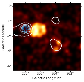
Finally we will combine both images in single plot, by plotting WMAP contours on top of the smoothed Fermi-LAT 2FHL image:
In [17]:
fig, ax, _ = vela_2fhl_cutout.plot()
ax.contour(vela_wmap_reprojected_cutout.data, cmap="Blues");
Exercises
- Add a marker and circle at the Vela pulsar position (you can find examples in the WCSAxes documentation).
Event lists
Almost any high-level gamma-ray data analysis starts with the raw measured counts data, which is stored in event lists. In Gammapy event lists are represented by the gammapy.data.EventList class.
In this section we will learn how to:
- Read event lists from FITS files
- Access and work with the
EventListattributes such as.tableand.energy - Filter events lists using convenience methods
Let’s start with the import from the gammapy.data submodule:
In [18]:
from gammapy.data import EventList
Very similar to the sky map class an event list can be created, by
passing a filename to the .read() method:
In [19]:
events_2fhl = EventList.read("$GAMMAPY_DATA/fermi_2fhl/2fhl_events.fits.gz")
This time the actual data is stored as an
astropy.table.Table
object. It can be accessed with .table attribute:
In [20]:
events_2fhl.table
Out[20]:
| ENERGY | RA | DEC | L | B | THETA | PHI | ZENITH_ANGLE | EARTH_AZIMUTH_ANGLE | TIME | EVENT_ID | RUN_ID | RECON_VERSION | CALIB_VERSION [3] | EVENT_CLASS [32] | EVENT_TYPE [32] | CONVERSION_TYPE | LIVETIME | DIFRSP0 | DIFRSP1 | DIFRSP2 | DIFRSP3 | DIFRSP4 |
|---|---|---|---|---|---|---|---|---|---|---|---|---|---|---|---|---|---|---|---|---|---|---|
| MeV | deg | deg | deg | deg | deg | deg | deg | deg | s | s | ||||||||||||
| float32 | float32 | float32 | float32 | float32 | float32 | float32 | float32 | float32 | float64 | int32 | int32 | int16 | int16 | bool | bool | int16 | float64 | float32 | float32 | float32 | float32 | float32 |
| 145927.0 | 291.662 | 42.2341 | 74.5437 | 11.8678 | 38.0455 | 83.5358 | 55.6387 | 314.034 | 239561457.866 | 4851437 | 239559565 | 0 | 0 .. 0 | False .. True | False .. True | 0 | 275.698088974 | 2.69657e-11 | 3238.25 | 0.0 | 0.0 | 0.0 |
| 221273.0 | 46.9858 | -40.6389 | 247.489 | -58.8739 | 34.1051 | 224.209 | 68.2524 | 198.319 | 239562739.085 | 7521432 | 239559565 | 0 | 0 .. 0 | False .. True | False .. True | 0 | 64.7974931598 | 1.53573e-12 | 2774.2 | 0.0 | 0.0 | 0.0 |
| 57709.2 | 121.841 | 49.2288 | 169.868 | 32.3017 | 71.5636 | 34.2925 | 36.7173 | 25.5439 | 239563180.302 | 8690693 | 239559565 | 0 | 0 .. 0 | False .. True | False .. True | 0 | 30.57218647 | 8.11096e-12 | 253.221 | 0.0 | 0.0 | 0.0 |
| 221224.0 | 83.5626 | -4.21744 | 207.783 | -19.0771 | 20.5089 | 92.1605 | 32.3033 | 239.141 | 239563382.213 | 9208424 | 239559565 | 0 | 0 .. 0 | False .. True | False .. True | 0 | 27.4125095904 | 1.66075e-11 | 2980.12 | 0.0 | 0.0 | 0.0 |
| 698997.0 | 320.895 | -1.32789 | 51.2218 | -33.9718 | 35.3621 | 158.741 | 12.0867 | 72.2029 | 239566572.951 | 2480483 | 239565645 | 0 | 0 .. 0 | False .. True | False .. True | 0 | 106.475481123 | 2.26543e-13 | 2706.14 | 0.0 | 0.0 | 0.0 |
| 119159.0 | 318.811 | 12.3028 | 62.6361 | -24.416 | 26.5896 | 213.894 | 17.7156 | 23.9409 | 239572348.06 | 1725276 | 239571670 | 0 | 0 .. 0 | False .. True | False .. True | 0 | 185.346427292 | 2.75677e-11 | 3439.29 | 0.0 | 0.0 | 0.0 |
| 56175.6 | 279.251 | 47.8835 | 76.6915 | 22.0739 | 29.1034 | 61.0048 | 62.1731 | 321.104 | 239572763.431 | 76017 | 239572736 | 0 | 0 .. 0 | False .. True | False .. True | 0 | 24.4507339597 | 2.08265e-10 | 4071.25 | 0.0 | 0.0 | 0.0 |
| 1.41812e+06 | 100.311 | -47.4481 | 256.468 | -21.2641 | 61.2256 | 294.18 | 90.4753 | 144.149 | 239573788.813 | 1781569 | 239572736 | 0 | 0 .. 0 | False .. True | False .. True | 0 | 68.271614641 | 3.20022e-14 | 1086.23 | 0.0 | 0.0 | 0.0 |
| 62164.9 | 331.492 | -41.2264 | 359.42 | -53.4049 | 28.1408 | 229.927 | 52.0142 | 189.054 | 239578601.168 | 2000700 | 239577663 | 0 | 0 .. 0 | False .. True | False .. True | 0 | 90.332262665 | 1.21479e-10 | 3566.07 | 0.0 | 0.0 | 0.0 |
| ... | ... | ... | ... | ... | ... | ... | ... | ... | ... | ... | ... | ... | ... | ... | ... | ... | ... | ... | ... | ... | ... | ... |
| 51296.8 | 79.0311 | 78.9327 | 133.868 | 22.2399 | 51.1726 | 267.814 | 99.7602 | 357.79 | 444418973.822 | 1284853 | 444418590 | 0 | 0 .. 0 | False .. True | False .. True | 0 | 181.6889835 | 2.14127e-10 | 2586.88 | 0.0 | 0.0 | 0.0 |
| 60315.7 | 243.681 | -50.5669 | 332.43 | 0.28268 | 24.8501 | 255.683 | 74.8804 | 195.14 | 444421777.761 | 6582949 | 444418590 | 0 | 0 .. 0 | False .. True | False .. False | 1 | 57.3358902931 | 2.35854e-08 | 3541.04 | 0.0 | 0.0 | 0.0 |
| 90000.1 | 282.698 | -33.1987 | 2.66219 | -14.3339 | 8.49144 | 343.559 | 47.3965 | 191.033 | 444422182.738 | 7507466 | 444418590 | 0 | 0 .. 0 | False .. True | False .. True | 0 | 187.602469146 | 3.62123e-10 | 3792.57 | 0.0 | 0.0 | 0.0 |
| 61988.7 | 247.98 | -48.1091 | 336.146 | 0.0220339 | 33.6499 | 144.271 | 80.3966 | 221.396 | 444422758.145 | 8699147 | 444418590 | 0 | 0 .. 0 | False .. True | False .. True | 0 | 39.2098327279 | 2.26421e-08 | 3395.07 | 0.0 | 0.0 | 0.0 |
| 54282.9 | 159.924 | -58.3628 | 286.362 | 0.205554 | 24.1196 | 287.138 | 65.0847 | 177.524 | 444425794.794 | 2522237 | 444424619 | 0 | 0 .. 0 | False .. True | False .. True | 0 | 196.209668875 | 4.8258e-09 | 3672.78 | 0.0 | 0.0 | 0.0 |
| 146728.0 | 244.848 | -46.5876 | 335.754 | 2.60326 | 45.2539 | 5.33644 | 91.871 | 137.032 | 444425911.819 | 2705210 | 444424619 | 0 | 0 .. 0 | False .. True | False .. False | 1 | 65.6327857375 | 4.4595e-10 | 2899.33 | 0.0 | 0.0 | 0.0 |
| 135433.0 | 83.5278 | 27.9053 | 179.529 | -2.69106 | 17.4911 | 52.0858 | 53.306 | 313.822 | 444430968.968 | 939188 | 444430599 | 0 | 0 .. 0 | False .. True | False .. False | 1 | 97.6446831226 | 1.57989e-10 | 3515.6 | 0.0 | 0.0 | 0.0 |
| 61592.1 | 231.214 | -5.45521 | 357.435 | 40.6473 | 46.6356 | 141.047 | 62.7584 | 256.631 | 444433607.906 | 5443944 | 444430599 | 0 | 0 .. 0 | False .. True | False .. False | 1 | 28.7290657759 | 2.82028e-10 | 2793.45 | 0.0 | 0.0 | 0.0 |
| 80480.8 | 228.244 | -45.044 | 327.561 | 10.9528 | 37.3149 | 193.714 | 83.3882 | 221.57 | 444433702.069 | 5612443 | 444430599 | 0 | 0 .. 0 | False .. True | False .. False | 1 | 122.891819298 | 2.26095e-10 | 3176.43 | 0.0 | 0.0 | 0.0 |
| 124449.0 | 238.008 | -51.0371 | 329.429 | 2.3006 | 32.4522 | 199.504 | 80.9768 | 214.48 | 444433764.433 | 5723361 | 444430599 | 0 | 0 .. 0 | False .. True | False .. True | 0 | 185.255487204 | 8.54908e-10 | 3366.3 | 0.0 | 0.0 | 0.0 |
Let’s try to find the total number of events contained int the list. This doesn’t work:
In [21]:
print("Total number of events: {}".format(len(events_2fhl.table)))
Total number of events: 60978
Because Gammapy objects don’t redefine properties, that are accessible from the underlying Astropy of Numpy data object.
So in this case of course we can directly use the .table attribute
to find the total number of events:
In [22]:
print("Total number of events: {}".format(len(events_2fhl.table)))
Total number of events: 60978
And we can access any other attribute of the Table object as well:
In [23]:
events_2fhl.table.colnames
Out[23]:
['ENERGY',
 'RA',
 'DEC',
 'L',
 'B',
 'THETA',
 'PHI',
 'ZENITH_ANGLE',
 'EARTH_AZIMUTH_ANGLE',
 'TIME',
 'EVENT_ID',
 'RUN_ID',
 'RECON_VERSION',
 'CALIB_VERSION',
 'EVENT_CLASS',
 'EVENT_TYPE',
 'CONVERSION_TYPE',
 'LIVETIME',
 'DIFRSP0',
 'DIFRSP1',
 'DIFRSP2',
 'DIFRSP3',
 'DIFRSP4']
For convenience we can access the most important event parameters as
properties on the EventList objects. The attributes will return
corresponding Astropy objects to represent the data, such as
astropy.units.Quantity,
astropy.coordinates.SkyCoord
or
astropy.time.Time
objects:
In [24]:
events_2fhl.energy.to("GeV")
Out[24]:
In [25]:
events_2fhl.galactic
# events_2fhl.radec
Out[25]:
<SkyCoord (Galactic): (l, b) in deg
    [(  74.54326949,  11.86794629), ( 247.48874019, -58.87409431),
     ( 169.86765712,  32.30144389), ..., ( 357.43496217,  40.64753602),
     ( 327.56037412,  10.95297324), ( 329.42901812,   2.30075607)]>
In [26]:
events_2fhl.time
Out[26]:
<Time object: scale='tt' format='mjd' value=[ 54682.7028015   54682.71763043  54682.72273711 ...,  57053.90824179
  57053.90933163  57053.91005343]>
In addition EventList provides convenience methods to filter the
event lists. One possible use case is to find the highest energy event
within a radius of 0.5 deg around the vela position:
In [27]:
# select all events within a radius of 0.5 deg around center
events_vela_2fhl = events_2fhl.select_sky_cone(
    center=center, radius=0.5 * u.deg
)

# sort events by energy
events_vela_2fhl.table.sort("ENERGY")

# and show highest energy photon
events_vela_2fhl.energy[-1].to("GeV")
Out[27]:
Exercises
- Make a counts energy spectrum for the galactic center region, within a radius of 10 deg.
Source catalogs
Gammapy provides a convenient interface to access and work with catalog based data.
In this section we will learn how to:
- Load builtins catalogs from gammapy.catalog
- Sort and index the underlying Astropy tables
- Access data from individual sources
Let’s start with importing the 2FHL catalog object from the gammapy.catalog submodule:
In [28]:
from gammapy.catalog import SourceCatalog2FHL
First we initialize the Fermi-LAT 2FHL catalog and directly take a look
at the .table attribute:
In [29]:
fermi_2fhl = SourceCatalog2FHL(
    "$GAMMAPY_DATA/catalogs/fermi/gll_psch_v08.fit.gz"
)
fermi_2fhl.table
Out[29]:
| Source_Name | RAJ2000 | DEJ2000 | GLON | GLAT | Pos_err_68 | TS | Spectral_Index | Unc_Spectral_Index | Intr_Spectral_Index_D11 | Unc_Intr_Spectral_Index_D11 | Intr_Spectral_Index_G12 | Unc_Intr_Spectral_Index_G12 | Flux50 | Unc_Flux50 | Energy_Flux50 | Unc_Energy_Flux50 | Flux50_171GeV | Unc_Flux50_171GeV [2] | Sqrt_TS50_171GeV | Flux171_585GeV | Unc_Flux171_585GeV [2] | Sqrt_TS171_585GeV | Flux585_2000GeV | Unc_Flux585_2000GeV [2] | Sqrt_TS585_2000GeV | Npred | HEP_Energy | HEP_Prob | ROI | ASSOC | ASSOC_PROB_BAY | ASSOC_PROB_LR | CLASS | Redshift | NuPeak_obs | 3FGL_Name | 1FHL_Name | TeVCat_Name |
|---|---|---|---|---|---|---|---|---|---|---|---|---|---|---|---|---|---|---|---|---|---|---|---|---|---|---|---|---|---|---|---|---|---|---|---|---|---|---|
| deg | deg | deg | deg | deg | 1 / (cm2 s) | 1 / (cm2 s) | erg / (cm2 s) | erg / (cm2 s) | 1 / (cm2 s) | 1 / (cm2 s) | 1 / (cm2 s) | 1 / (cm2 s) | 1 / (cm2 s) | 1 / (cm2 s) | GeV | Hz | ||||||||||||||||||||||
| bytes18 | float32 | float32 | float32 | float32 | float32 | float32 | float32 | float32 | float32 | float32 | float32 | float32 | float32 | float32 | float32 | float32 | float32 | float32 | float32 | float32 | float32 | float32 | float32 | float32 | float32 | float32 | float32 | float32 | int16 | bytes25 | float32 | float32 | bytes8 | float32 | float32 | bytes18 | bytes18 | bytes18 |
| 2FHL J0008.1+4709 | 2.0437 | 47.1642 | 115.339 | -15.0688 | 0.061114 | 28.64 | 6.24 | 2.75 | 3.96 | 3.19 | 2.16 | 4.21 | 1.23e-11 | 6.71e-12 | 1.21e-12 | 6.71e-13 | 3.36344e-12 | -1.53668e-12 .. 2.16095e-12 | 5.35354 | 4.34947e-18 | nan .. 4.75389e-12 | 0.0 | 8.44871e-18 | nan .. 7.29101e-12 | 0.0 | 4.0 | 68.15 | 0.99 | 1 | MG4 J000800+4712 | 0.99722 | 0.834827 | bll | 2.1 | 2.51188e+15 | 3FGL J0008.0+4713 | 1FHL J0007.7+4709 | |
| 2FHL J0009.3+5031 | 2.3435 | 50.5217 | 116.124 | -11.7932 | 0.0454392 | 53.97 | 5.08 | 1.66 | nan | nan | nan | nan | 1.91e-11 | 7.82e-12 | 2.03e-12 | 8.79e-13 | 8.36282e-12 | -2.98962e-12 .. 3.89512e-12 | 7.35132 | 2.91458e-17 | nan .. 5.10003e-12 | 0.0 | 3.50875e-16 | nan .. 4.87458e-12 | 0.0 | 6.4 | 72.76 | 1.0 | 1 | NVSS J000922+503028 | 0.999724 | 0.734808 | bll | 0.0 | 1.41254e+15 | 3FGL J0009.3+5030 | 1FHL J0009.2+5032 | |
| 2FHL J0018.5+2947 | 4.6355 | 29.7879 | 114.463 | -32.5424 | 0.0370936 | 30.89 | 2.58 | 0.99 | 2.41 | 1.04 | 2.4 | 1.04 | 1.06e-11 | 6.15e-12 | 2.05e-12 | 1.72e-12 | 9.65438e-12 | -5.55342e-12 .. 5.55342e-12 | 5.76579 | 1.179e-15 | nan .. 5.37865e-12 | 0.0 | 1.60465e-16 | nan .. 6.12008e-12 | 0.0 | 3.0 | 127.32 | 1.0 | 3 | RBS 0042 | 0.999868 | 0.978522 | bll | 0.1 | 5.91561e+16 | 3FGL J0018.4+2947 | 1FHL J0018.6+2946 | |
| 2FHL J0022.0+0006 | 5.5001 | 0.1059 | 107.172 | -61.8618 | 0.0511852 | 29.96 | 1.86 | 0.57 | 0.95 | 0.72 | 0.88 | 0.71 | 1.97e-11 | 9.56e-12 | 6.86e-12 | 5.29e-12 | 1.61197e-11 | -7.17255e-12 .. 9.95349e-12 | 5.3822 | 3.63922e-12 | -4.38636e-12 .. 4.38636e-12 | 1.38539 | 8.42356e-16 | nan .. 7.3424e-12 | 0.0 | 4.8 | 180.13 | 0.86 | 2 | 5BZGJ0022+0006 | 0.99928 | 0.900089 | bll-g | 0.306 | 4.31519e+16 | |||
| 2FHL J0033.6-1921 | 8.4115 | -19.3575 | 94.28 | -81.2224 | 0.0348384 | 148.31 | 3.32 | 0.69 | 2.56 | 0.88 | 2.33 | 0.92 | 5.46e-11 | 1.5e-11 | 7.62e-12 | 2.69e-12 | 4.00161e-11 | -1.01615e-11 .. 1.22378e-11 | 12.1725 | 2.13901e-12 | nan .. 8.25812e-12 | 0.907958 | 2.43955e-17 | nan .. 6.84226e-12 | 0.0 | 13.8 | 170.01 | 0.99 | 2 | KUV 00311-1938 | 0.999759 | 0.981424 | bll | 0.61 | 8.31764e+15 | 3FGL J0033.6-1921 | 1FHL J0033.6-1921 | TeV J0033-1921 |
| 2FHL J0035.8+5949 | 8.9625 | 59.8312 | 120.972 | -2.98122 | 0.0316026 | 402.4 | 2.23 | 0.21 | nan | nan | nan | nan | 1.25e-10 | 1.9e-11 | 3.11e-11 | 7.23e-12 | 9.42294e-11 | -1.52566e-11 .. 1.71572e-11 | 17.3124 | 2.66991e-11 | -7.62818e-12 .. 9.45084e-12 | 10.3909 | 3.72609e-16 | nan .. 4.67444e-12 | 0.0 | 46.5 | 247.62 | 0.96 | 4 | 1ES 0033+595 | 0.999958 | 0.992868 | bll | 0.0 | 1.31826e+17 | 3FGL J0035.9+5949 | 1FHL J0035.9+5950 | TeV J0035+5950 |
| 2FHL J0040.3+4049 | 10.0949 | 40.8315 | 120.676 | -21.9918 | 0.0355148 | 26.76 | 2.12 | 0.81 | nan | nan | nan | nan | 1.05e-11 | 6.3e-12 | 2.84e-12 | 2.67e-12 | 7.41577e-12 | -4.0778e-12 .. 6.45182e-12 | 4.95442 | 3.00308e-12 | -2.31775e-12 .. 4.46644e-12 | 1.70835 | 4.73166e-16 | nan .. 5.79809e-12 | 0.0 | 3.2 | 258.77 | 0.85 | 3 | B3 0037+405 | 0.998738 | 0.9347 | bcu I | 0.0 | 1.0 | 3FGL J0040.3+4049 | 1FHL J0040.3+4049 | |
| 2FHL J0043.9+3424 | 10.9755 | 34.4109 | 121.164 | -28.435 | 0.0592417 | 39.5 | 4.57 | 1.61 | 3.46 | 1.85 | 2.95 | 1.91 | 1.83e-11 | 8.24e-12 | 2.03e-12 | 9.93e-13 | 9.65762e-12 | -4.31687e-12 .. 4.31687e-12 | 6.31152 | 8.75861e-17 | nan .. 5.24335e-12 | 0.0 | 9.43812e-16 | nan .. 5.68787e-12 | 0.0 | 5.4 | 109.97 | 0.9 | 3 | GB6 J0043+3426 | 0.998594 | 0.838844 | fsrq | 0.966 | 6.45655e+13 | 3FGL J0043.8+3425 | 1FHL J0043.7+3425 | |
| 2FHL J0045.2+2127 | 11.3161 | 21.4555 | 121.017 | -41.3933 | 0.0378046 | 110.43 | 3.07 | 0.64 | nan | nan | nan | nan | 4.14e-11 | 1.26e-11 | 6.29e-12 | 2.45e-12 | 3.11532e-11 | -8.93008e-12 .. 1.10103e-11 | 10.2404 | 2.99712e-12 | -3.03054e-12 .. 3.03054e-12 | 2.7089 | 4.68348e-17 | nan .. 6.42314e-12 | 0.0 | 11.4 | 246.75 | 0.99 | 5 | GB6 J0045+2127 | 0.99961 | 0.965127 | bll | 0.0 | 1.0023e+16 | 3FGL J0045.3+2126 | 1FHL J0045.2+2126 | |
| ... | ... | ... | ... | ... | ... | ... | ... | ... | ... | ... | ... | ... | ... | ... | ... | ... | ... | ... | ... | ... | ... | ... | ... | ... | ... | ... | ... | ... | ... | ... | ... | ... | ... | ... | ... | ... | ... | ... |
| 2FHL J2322.5+3436 | 350.628 | 34.613 | 102.876 | -24.7718 | 0.0717998 | 28.77 | 2.33 | 0.8 | 2.13 | 0.85 | 2.11 | 0.85 | 1.42e-11 | 7.46e-12 | 3.24e-12 | 2.48e-12 | 1.37062e-11 | -5.99053e-12 .. 8.27325e-12 | 5.51109 | 1.50445e-15 | nan .. 5.25568e-12 | 0.0 | 3.34396e-16 | nan .. 6.35236e-12 | 0.0 | 4.1 | 166.2 | 0.99 | 133 | TXS 2320+343 | 0.996639 | 0.877901 | bll-g | 0.098 | 1.04713e+15 | 3FGL J2322.5+3436 | 1FHL J2322.5+3436 | |
| 2FHL J2322.7-4916 | 350.698 | -49.2706 | 334.608 | -62.0492 | 0.038949 | 36.84 | 4.58 | 1.69 | nan | nan | nan | nan | 1.75e-11 | 8.3e-12 | 1.94e-12 | 9.96e-13 | 9.13009e-12 | -3.73356e-12 .. 5.01738e-12 | 6.05223 | 6.65757e-17 | nan .. 5.27137e-12 | 0.0 | 6.34713e-16 | nan .. 5.77243e-12 | 0.0 | 5.1 | 106.33 | 0.9 | 138 | SUMSS J232254-491629 | 0.999434 | 0.937726 | bll | 0.0 | 4.46683e+15 | 3FGL J2322.9-4917 | ||
| 2FHL J2323.4+5848 | 350.874 | 58.808 | 111.744 | -2.14031 | 0.0348384 | 183.62 | 2.45 | 0.3 | nan | nan | nan | nan | 7.81e-11 | 1.53e-11 | 1.64e-11 | 4.68e-12 | 5.93689e-11 | -1.21101e-11 .. 1.38986e-11 | 11.6238 | 1.03761e-11 | -4.37845e-12 .. 6.14398e-12 | 5.81435 | 2.90309e-12 | -2.02416e-12 .. 3.98202e-12 | 3.50834 | 28.8 | 662.12 | 1.0 | 135 | Cas A | nan | 0.999833 | snr | nan | nan | 3FGL J2323.4+5849 | 1FHL J2323.3+5849 | TeV J2323+588 |
| 2FHL J2323.8+4209 | 350.972 | 42.1629 | 106.059 | -17.8224 | 0.0456016 | 70.61 | 4.21 | 1.16 | 4.14 | 1.15 | 4.13 | 1.15 | 3.05e-11 | 1.05e-11 | 3.55e-12 | 1.35e-12 | 1.62017e-11 | -5.24708e-12 .. 6.61912e-12 | 8.11938 | 2.00018e-12 | -1.41271e-12 .. 2.77927e-12 | 2.56849 | 2.18906e-18 | nan .. 5.54082e-12 | 0.0 | 9.3 | 230.9 | 0.92 | 133 | 1ES 2321+419 | 0.99956 | 0.961506 | bll | 0.059 | 4.84173e+15 | 3FGL J2323.9+4211 | 1FHL J2323.8+4210 | |
| 2FHL J2324.7-4041 | 351.195 | -40.6934 | 350.157 | -67.5836 | 0.0358658 | 80.93 | 3.18 | 0.83 | 2.94 | 0.87 | 2.9 | 0.87 | 2.97e-11 | 1.08e-11 | 4.34e-12 | 2.03e-12 | 2.13391e-11 | -7.09939e-12 .. 9.10435e-12 | 8.85383 | 2.71834e-12 | -2.11714e-12 .. 4.11668e-12 | 1.65792 | 3.54717e-17 | nan .. 6.3514e-12 | 0.0 | 8.0 | 118.48 | 1.0 | 138 | 1ES 2322-409 | 0.999467 | 0.985516 | bll | 0.173587 | 8.31764e+15 | 3FGL J2324.7-4040 | 1FHL J2324.6-4041 | |
| 2FHL J2329.2+3754 | 352.308 | 37.9157 | 105.532 | -22.1627 | 0.038539 | 39.4 | 3.29 | 1.19 | 2.99 | 1.28 | 2.92 | 1.28 | 1.43e-11 | 7.17e-12 | 2.02e-12 | 1.25e-12 | 1.11304e-11 | -4.6962e-12 .. 6.5288e-12 | 6.31149 | 4.40415e-16 | nan .. 5.47737e-12 | 0.0 | 2.64065e-17 | nan .. 5.92547e-12 | 0.0 | 4.3 | 142.13 | 0.98 | 133 | NVSS J232914+375414 | 0.999792 | 0.956363 | bll | 0.264 | 8.91251e+15 | 3FGL J2329.2+3754 | 1FHL J2329.1+3754 | |
| 2FHL J2340.8+8014 | 355.203 | 80.2447 | 119.838 | 17.7999 | 0.0348934 | 69.79 | 4.2 | 1.28 | 4.0 | 1.36 | 3.94 | 1.37 | 1.95e-11 | 7.24e-12 | 2.26e-12 | 9.72e-13 | 1.16398e-11 | -3.81183e-12 .. 4.82791e-12 | 8.38745 | 1.25703e-16 | nan .. 3.71812e-12 | 0.0 | 1.13621e-15 | nan .. 4.04723e-12 | 0.0 | 7.9 | 80.85 | 0.86 | 125 | 1RXS J234051.4+801513 | 0.999874 | 0.979435 | bll | 0.274 | 3.42768e+15 | 3FGL J2340.7+8016 | 1FHL J2341.3+8016 | |
| 2FHL J2343.5+3438 | 355.898 | 34.6484 | 107.422 | -26.1717 | 0.0715056 | 27.43 | 4.99 | 2.36 | 4.88 | 2.43 | 4.79 | 2.44 | 1.33e-11 | 7.32e-12 | 1.41e-12 | 8.56e-13 | 5.94254e-12 | -2.73222e-12 .. 3.85247e-12 | 5.2347 | 5.08627e-17 | nan .. 8.36317e-12 | 0.0 | 3.14709e-16 | nan .. 5.6852e-12 | 0.0 | 3.9 | 72.66 | 1.0 | 133 | 1RXS J234332.5+343957 | 0.999148 | 0.955429 | bll | 0.366 | 1.0292e+15 | 3FGL J2343.7+3437 | ||
| 2FHL J2347.1+5142 | 356.75 | 51.7081 | 112.88 | -9.90159 | 0.0335464 | 209.84 | 1.85 | 0.25 | 1.74 | 0.26 | 1.73 | 0.26 | 7.48e-11 | 1.54e-11 | 2.62e-11 | 8.56e-12 | 4.78884e-11 | -1.15596e-11 .. 1.339e-11 | 11.282 | 2.42894e-11 | -7.68104e-12 .. 9.87777e-12 | 8.8577 | 3.51388e-12 | -3.55282e-12 .. 3.55282e-12 | 2.66572 | 25.2 | 652.31 | 0.99 | 1 | 1ES 2344+514 | 0.99986 | 0.988082 | bll | 0.044 | 7.07946e+15 | 3FGL J2347.0+5142 | 1FHL J2347.0+5142 | TeV J2346+5142 |
| 2FHL J2352.0-7558 | 358.019 | -75.9718 | 307.623 | -40.6111 | 0.0733733 | 28.49 | 3.37 | 1.24 | nan | nan | nan | nan | 1.18e-11 | 6.14e-12 | 1.63e-12 | 1.03e-12 | 9.00308e-12 | -3.9133e-12 .. 5.47729e-12 | 5.38935 | 3.90782e-16 | nan .. 4.95279e-12 | 0.0 | 3.23398e-17 | nan .. 5.16722e-12 | 0.0 | 3.9 | 134.72 | 1.0 | 137 | nan | nan | unk | nan | nan | 3FGL J2351.9-7601 |
This looks very familiar again. The data is just stored as an
astropy.table.Table
object. We have all the methods and attributes of the Table object
available. E.g. we can sort the underlying table by TS to find the
top 5 most significant sources:
In [30]:
# sort table by TS
fermi_2fhl.table.sort("TS")

# invert the order to find the highest values and take the top 5
top_five_TS_2fhl = fermi_2fhl.table[::-1][:5]

# print the top five significant sources with association and source class
top_five_TS_2fhl[["Source_Name", "ASSOC", "CLASS"]]
Out[30]:
| Source_Name | ASSOC | CLASS |
|---|---|---|
| bytes18 | bytes25 | bytes8 |
| 2FHL J1104.4+3812 | Mkn 421 | bll |
| 2FHL J0534.5+2201 | Crab | pwn |
| 2FHL J1653.9+3945 | Mkn 501 | bll |
| 2FHL J1555.7+1111 | PG 1553+113 | bll |
| 2FHL J2158.8-3013 | PKS 2155-304 | bll |
If you are interested in the data of an individual source you can access the information from catalog using the name of the source or any alias source name that is defined in the catalog:
In [31]:
mkn_421_2fhl = fermi_2fhl["2FHL J1104.4+3812"]

# or use any alias source name that is defined in the catalog
mkn_421_2fhl = fermi_2fhl["Mkn 421"]
print(mkn_421_2fhl.data["TS"])
5600.98
Exercises
- Try to load the Fermi-LAT 3FHL catalog and check the total number of sources it contains.
- Select all the sources from the 2FHL catalog which are contained in the Vela region. Add markers for all these sources and try to add labels with the source names. The function ax.text() might be helpful.
- Try to find the source class of the object at position ra=68.6803, dec=9.3331
Spectral models and flux points
In the previous section we learned how access basic data from individual sources in the catalog. Now we will go one step further and explore the full spectral information of sources. We will learn how to:
- Plot spectral models
- Compute integral and energy fluxes
- Read and plot flux points
As a first example we will start with the Crab Nebula:
In [32]:
crab_2fhl = fermi_2fhl["Crab"]
print(crab_2fhl.spectral_model)
PowerLaw2

Parameters:

           name     value     error       unit    min max
        --------- --------- --------- ----------- --- ---
        amplitude 1.310e-09 6.830e-11 1 / (cm2 s) nan nan
            index 2.130e+00 7.000e-02             nan nan
             emin 5.000e-02 0.000e+00         TeV nan nan
             emax 2.000e+00 0.000e+00         TeV nan nan

Covariance:

           name   amplitude   index      emin      emax
        --------- --------- --------- --------- ---------
        amplitude 4.665e-21 0.000e+00 0.000e+00 0.000e+00
            index 0.000e+00 4.900e-03 0.000e+00 0.000e+00
             emin 0.000e+00 0.000e+00 0.000e+00 0.000e+00
             emax 0.000e+00 0.000e+00 0.000e+00 0.000e+00
The crab_2fhl.spectral_model is an instance of the
gammapy.spectrum.models.PowerLaw2
model, with the parameter values and errors taken from the 2FHL catalog.
Let’s plot the spectral model in the energy range between 50 GeV and 2000 GeV:
In [33]:
ax_crab_2fhl = crab_2fhl.spectral_model.plot(
    energy_range=[50, 2000] * u.GeV, energy_power=0
)
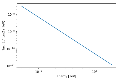
We assign the return axes object to variable called ax_crab_2fhl,
because we will re-use it later to plot the flux points on top.
To compute the differential flux at 100 GeV we can simply call the model like normal Python function and convert to the desired units:
In [34]:
crab_2fhl.spectral_model(100 * u.GeV).to("cm-2 s-1 GeV-1")
Out[34]:
Next we can compute the integral flux of the Crab between 50 GeV and 2000 GeV:
In [35]:
crab_2fhl.spectral_model.integral(emin=50 * u.GeV, emax=2000 * u.GeV).to(
    "cm-2 s-1"
)
Out[35]:
We can easily convince ourself, that it corresponds to the value given in the Fermi-LAT 2FHL catalog:
In [36]:
crab_2fhl.data["Flux50"]
Out[36]:
In addition we can compute the energy flux between 50 GeV and 2000 GeV:
In [37]:
crab_2fhl.spectral_model.energy_flux(emin=50 * u.GeV, emax=2000 * u.GeV).to(
    "erg cm-2 s-1"
)
Out[37]:
Next we will access the flux points data of the Crab:
In [38]:
print(crab_2fhl.flux_points)
FluxPoints(sed_type="dnde", n_points=3)
If you want to learn more about the different flux point formats you can read the specification here.
No we can check again the underlying astropy data structure by accessing
the .table attribute:
In [39]:
crab_2fhl.flux_points.table
Out[39]:
| e_min | e_max | flux | flux_errn | flux_errp | is_ul | flux_ul | e_ref | dnde | dnde_errn | dnde_errp | dnde_ul |
|---|---|---|---|---|---|---|---|---|---|---|---|
| GeV | GeV | 1 / (cm2 s) | 1 / (cm2 s) | 1 / (cm2 s) | 1 / (cm2 s) | GeV | 1 / (cm2 GeV s) | 1 / (cm2 GeV s) | 1 / (cm2 GeV s) | 1 / (cm2 GeV s) | |
| float64 | float64 | float64 | float32 | float32 | bool | float64 | float64 | float64 | float64 | float64 | float64 |
| 50.0 | 171.0 | 9.940720469e-10 | 5.7595e-11 | 5.94726e-11 | False | nan | 92.4662100445 | 8.07727825726e-12 | 4.67985048251e-13 | 4.83241713057e-13 | nan |
| 171.0 | 585.0 | 2.43875392103e-10 | 2.82542e-11 | 3.04354e-11 | False | nan | 316.283101035 | 5.79157393348e-13 | 6.70984284998e-14 | 7.22782614849e-14 | nan |
| 585.0 | 2000.0 | 5.27535862216e-11 | 1.33401e-11 | 1.60478e-11 | False | nan | 1081.66538264 | 3.66549119269e-14 | 9.26915205272e-15 | 1.11505059757e-14 | nan |
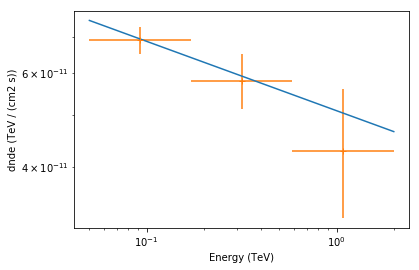
Finally let’s combine spectral model and flux points in a single plot
and scale with energy_power=2 to obtain the spectral energy
distribution:
In [40]:
ax = crab_2fhl.spectral_model.plot(
    energy_range=[50, 2000] * u.GeV, energy_power=2
)
crab_2fhl.flux_points.plot(ax=ax, energy_power=2);
Exercises
- Plot the spectral model and flux points for PKS 2155-304 for the 3FGL and 2FHL catalogs. Try to plot the error of the model (aka “Butterfly”) as well. Note this requires the uncertainties package to be installed on your machine.
What next?
This was a quick introduction to some of the high-level classes in Astropy and Gammapy.
- To learn more about those classes, go to the API docs (links are in the introduction at the top).
- To learn more about other parts of Gammapy (e.g. Fermi-LAT and TeV data analysis), check out the other tutorial notebooks.
- To see what’s available in Gammapy, browse the Gammapy docs or use the full-text search.
- If you have any questions, ask on the mailing list.