This is a fixed-text formatted version of a Jupyter notebook.
- Try online

- You can contribute with your own notebooks in this GitHub repository.
- Source files: cta_data_analysis.ipynb | cta_data_analysis.py

CTA first data challenge logo
CTA data analysis with Gammapy
Introduction
This notebook shows an example how to make a sky image and spectrum for simulated CTA data with Gammapy.
The dataset we will use is three observation runs on the Galactic center. This is a tiny (and thus quick to process and play with and learn) subset of the simulated CTA dataset that was produced for the first data challenge in August 2017.
This notebook can be considered part 2 of the introduction to CTA 1DC analysis. Part one is here: `cta_1dc_introduction.ipynb <cta_1dc_introduction.ipynb>`__
Setup
As usual, we’ll start with some setup …
In [1]:
%matplotlib inline
import matplotlib.pyplot as plt
In [2]:
!gammapy info --no-envvar --no-system
Gammapy package:

        path                   : /Users/jer/git/gammapy/gammapy
        version                : 0.8


Other packages:

        numpy                  : 1.13.0
        scipy                  : 0.19.1
        matplotlib             : 2.2.3
        cython                 : 0.28.5
        astropy                : 3.0.4
        astropy_healpix        : 0.2
        reproject              : 0.4
        sherpa                 : 4.10.0
        pytest                 : 3.7.1
        sphinx                 : 1.7.6
        healpy                 : 1.11.0
        regions                : 0.3
        iminuit                : 1.3.2
        naima                  : 0.8.1
        uncertainties          : 3.0.2
In [3]:
import numpy as np
import astropy.units as u
from astropy.coordinates import SkyCoord, Angle
from astropy.convolution import Gaussian2DKernel
from regions import CircleSkyRegion
from gammapy.utils.energy import EnergyBounds
from gammapy.data import DataStore
from gammapy.spectrum import (
    SpectrumExtraction,
    SpectrumFit,
    SpectrumResult,
    models,
    SpectrumEnergyGroupMaker,
    FluxPointEstimator,
)
from gammapy.maps import Map, MapAxis, WcsNDMap, WcsGeom
from gammapy.cube import MapMaker
from gammapy.background import ReflectedRegionsBackgroundEstimator
from gammapy.detect import TSMapEstimator, find_peaks
In [4]:
# Configure the logger, so that the spectral analysis
# isn't so chatty about what it's doing.
import logging

logging.basicConfig()
log = logging.getLogger("gammapy.spectrum")
log.setLevel(logging.ERROR)
Select observations
Like explained in
cta_1dc_introduction.ipynb, a Gammapy
analysis usually starts by creating a DataStore and selecting
observations.
This is shown in detail in the other notebook, here we just pick three observations near the galactic center.
In [5]:
data_store = DataStore.from_dir("$GAMMAPY_DATA/cta-1dc/index/gps")
In [6]:
# Just as a reminder: this is how to select observations
# from astropy.coordinates import SkyCoord
# table = data_store.obs_table
# pos_obs = SkyCoord(table['GLON_PNT'], table['GLAT_PNT'], frame='galactic', unit='deg')
# pos_target = SkyCoord(0, 0, frame='galactic', unit='deg')
# offset = pos_target.separation(pos_obs).deg
# mask = (1 < offset) & (offset < 2)
# table = table[mask]
# table.show_in_browser(jsviewer=True)
In [7]:
obs_id = [110380, 111140, 111159]
obs_list = data_store.obs_list(obs_id)
In [8]:
obs_cols = ["OBS_ID", "GLON_PNT", "GLAT_PNT", "LIVETIME"]
data_store.obs_table.select_obs_id(obs_id)[obs_cols]
Out[8]:
| OBS_ID | GLON_PNT | GLAT_PNT | LIVETIME |
|---|---|---|---|
| int64 | float64 | float64 | float64 |
| 110380 | 359.999991204 | -1.29999593791 | 1764.0 |
| 111140 | 358.499983383 | 1.3000020212 | 1764.0 |
| 111159 | 1.50000565683 | 1.29994046834 | 1764.0 |
Make sky images
Define map geometry
Select the target position and define an ON region for the spectral analysis
In [9]:
axis = MapAxis.from_edges(
    np.logspace(-1., 1., 10), unit="TeV", name="energy", interp="log"
)
geom = WcsGeom.create(
    skydir=(0, 0), npix=(500, 400), binsz=0.02, coordsys="GAL", axes=[axis]
)
geom
Out[9]:
WcsGeom

    axes       : lon, lat, energy
    shape      : (500, 400, 9)
    ndim       : 3
    coordsys   : GAL
    projection : CAR
    center     : 0.0 deg, 0.0 deg
    width      : 10.0 x 8.0 deg
Compute images
Exclusion mask currently unused. Remove here or move to later in the tutorial?
In [10]:
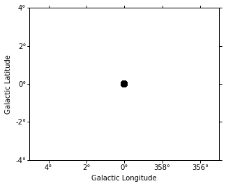
target_position = SkyCoord(0, 0, unit="deg", frame="galactic")
on_radius = 0.2 * u.deg
on_region = CircleSkyRegion(center=target_position, radius=on_radius)
In [11]:
exclusion_mask = geom.to_image().region_mask([on_region], inside=False)
exclusion_mask = WcsNDMap(geom.to_image(), exclusion_mask)
exclusion_mask.plot();
In [12]:
%%time
maker = MapMaker(geom, offset_max="2 deg")
maps = maker.run(obs_list)
print(maps.keys())
dict_keys(['counts', 'exposure', 'background'])
CPU times: user 4.24 s, sys: 687 ms, total: 4.93 s
Wall time: 4.94 s
In [13]:
# The maps are cubes, with an energy axis.
# Let's also make some images:
images = maker.make_images()

excess = images["counts"].copy()
excess.data -= images["background"].data
images["excess"] = excess
Show images
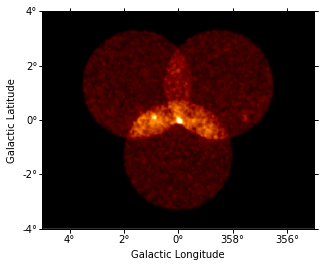
Let’s have a quick look at the images we computed …
In [14]:
images["counts"].smooth(2).plot(vmax=5);
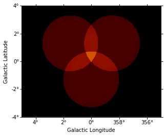
In [15]:
images["background"].plot(vmax=5);
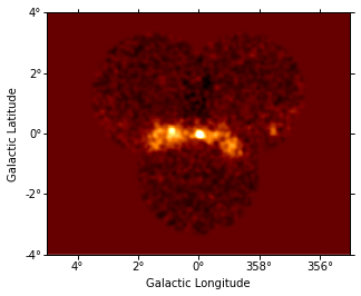
In [16]:
images["excess"].smooth(3).plot(vmax=2);
Source Detection
Use the class gammapy.detect.TSMapEstimator and gammapy.detect.find_peaks to detect sources on the images:
In [17]:
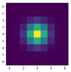
kernel = Gaussian2DKernel(1, mode="oversample").array
plt.imshow(kernel);
In [18]:
%%time
ts_image_estimator = TSMapEstimator()
images_ts = ts_image_estimator.run(images, kernel)
print(images_ts.keys())
dict_keys(['ts', 'sqrt_ts', 'flux', 'flux_err', 'flux_ul', 'niter'])
CPU times: user 740 ms, sys: 146 ms, total: 886 ms
Wall time: 10.4 s
In [19]:
sources = find_peaks(images_ts["sqrt_ts"], threshold=8)
sources
Out[19]:
| value | x | y | ra | dec |
|---|---|---|---|---|
| deg | deg | |||
| float32 | int64 | int64 | float64 | float64 |
| 19.798 | 252 | 197 | 266.42400 | -29.00490 |
| 8.9666 | 207 | 204 | 266.82019 | -28.16314 |
In [20]:
source_pos = SkyCoord(sources["ra"], sources["dec"])
source_pos
Out[20]:
<SkyCoord (ICRS): (ra, dec) in deg
    [( 266.42399798, -29.00490483), ( 266.82018801, -28.16313964)]>
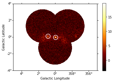
In [21]:
# Plot sources on top of significance sky image
images_ts["sqrt_ts"].plot(add_cbar=True)

plt.gca().scatter(
    source_pos.ra.deg,
    source_pos.dec.deg,
    transform=plt.gca().get_transform("icrs"),
    color="none",
    edgecolor="white",
    marker="o",
    s=200,
    lw=1.5,
);
Spatial analysis
See other notebooks for how to run a 3D cube or 2D image based analysis.
Spectrum
We’ll run a spectral analysis using the classical reflected regions background estimation method, and using the on-off (often called WSTAT) likelihood function.
Extraction
The first step is to “extract” the spectrum, i.e. 1-dimensional counts and exposure and background vectors, as well as an energy dispersion matrix from the data and IRFs.
In [22]:
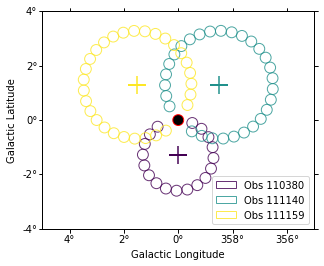
%%time
bkg_estimator = ReflectedRegionsBackgroundEstimator(
    obs_list=obs_list, on_region=on_region, exclusion_mask=exclusion_mask
)
bkg_estimator.run()
bkg_estimate = bkg_estimator.result
bkg_estimator.plot();
/Users/jer/anaconda/envs/gammapy-dev/lib/python3.6/site-packages/matplotlib/patches.py:83: UserWarning: Setting the 'color' property will overridethe edgecolor or facecolor properties.
  warnings.warn("Setting the 'color' property will override"
CPU times: user 5.37 s, sys: 241 ms, total: 5.61 s
Wall time: 5.66 s
In [23]:
%%time
extract = SpectrumExtraction(obs_list=obs_list, bkg_estimate=bkg_estimate)
extract.run()
observations = extract.observations
CPU times: user 849 ms, sys: 14.4 ms, total: 864 ms
Wall time: 868 ms
Model fit
The next step is to fit a spectral model, using all data (i.e. a “global” fit, using all energies).
In [24]:
%%time
model = models.PowerLaw(
    index=2, amplitude=1e-11 * u.Unit("cm-2 s-1 TeV-1"), reference=1 * u.TeV
)
fit = SpectrumFit(observations, model)
fit.run()
print(fit.result[0])
Fit result info
---------------
Model: PowerLaw

Parameters:

           name     value     error         unit         min    max
        --------- --------- --------- --------------- --------- ---
            index 2.225e+00 2.616e-02                       nan nan
        amplitude 3.013e-12 1.396e-13 1 / (cm2 s TeV)       nan nan
        reference 1.000e+00 0.000e+00             TeV 0.000e+00 nan

Covariance:

           name     index    amplitude  reference
        --------- ---------- ---------- ---------
            index  6.842e-04 -9.885e-16 0.000e+00
        amplitude -9.885e-16  1.950e-26 0.000e+00
        reference  0.000e+00  0.000e+00 0.000e+00

Statistic: 91.148 (wstat)
Fit Range: [  1.00000000e-02   1.00000000e+02] TeV

CPU times: user 360 ms, sys: 6.28 ms, total: 366 ms
Wall time: 366 ms
Spectral points
Finally, let’s compute spectral points. The method used is to first choose an energy binning, and then to do a 1-dim likelihood fit / profile to compute the flux and flux error.
In [25]:
# Flux points are computed on stacked observation
stacked_obs = extract.observations.stack()
print(stacked_obs)
*** Observation summary report ***
Observation Id: [110380-111159]
Livetime: 1.470 h
On events: 2377
Off events: 34876
Alpha: 0.041
Bkg events in On region: 1435.66
Excess: 941.34
Excess / Background: 0.66
Gamma rate: 0.18 1 / s
Bkg rate: 0.23 1 / min
Sigma: 22.14
energy range: 0.01 TeV - 100.00 TeV
In [26]:
ebounds = EnergyBounds.equal_log_spacing(1, 40, 4, unit=u.TeV)

seg = SpectrumEnergyGroupMaker(obs=stacked_obs)
seg.compute_groups_fixed(ebounds=ebounds)

fpe = FluxPointEstimator(
    obs=stacked_obs, groups=seg.groups, model=fit.result[0].model
)
fpe.compute_points()
fpe.flux_points.table
Out[26]:
| e_ref | e_min | e_max | dnde | dnde_err | dnde_ul | is_ul | sqrt_ts | dnde_errp | dnde_errn |
|---|---|---|---|---|---|---|---|---|---|
| TeV | TeV | TeV | 1 / (cm2 s TeV) | 1 / (cm2 s TeV) | 1 / (cm2 s TeV) | 1 / (cm2 s TeV) | 1 / (cm2 s TeV) | ||
| float64 | float64 | float64 | float64 | float64 | float64 | bool | float64 | float64 | float64 |
| 1.56474814166 | 1.0 | 2.44843674682 | 1.09665927288e-12 | 1.2341157896e-13 | 1.35849249895e-12 | False | 13.8584822281 | nan | nan |
| 3.83118684956 | 2.44843674682 | 5.99484250319 | 1.57243008959e-13 | 1.9436004648e-14 | 1.98486309052e-13 | False | 13.7091592194 | nan | nan |
| 10.0 | 5.99484250319 | 16.681005372 | 1.19005011546e-14 | 2.6277413917e-15 | 1.78643655366e-14 | False | 7.46562284258 | nan | nan |
| 26.1015721568 | 16.681005372 | 40.8423865267 | 7.4706997312e-16 | 4.14358281946e-16 | 1.83474469974e-15 | False | 2.75570747694 | nan | nan |
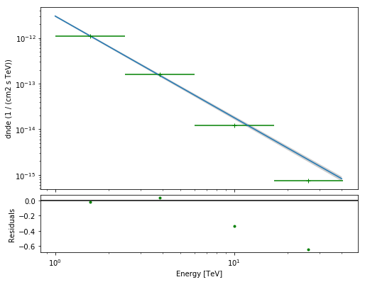
Plot
Let’s plot the spectral model and points. You could do it directly, but there is a helper class. Note that a spectral uncertainty band, a “butterfly” is drawn, but it is very thin, i.e. barely visible.
In [27]:
total_result = SpectrumResult(
    model=fit.result[0].model, points=fpe.flux_points
)

total_result.plot(
    energy_range=[1, 40] * u.TeV,
    fig_kwargs=dict(figsize=(8, 8)),
    point_kwargs=dict(color="green"),
);
Exercises
- Re-run the analysis above, varying some analysis parameters, e.g.
- Select a few other observations
- Change the energy band for the map
- Change the spectral model for the fit
- Change the energy binning for the spectral points
- Change the target. Make a sky image and spectrum for your favourite
source.
- If you don’t know any, the Crab nebula is the “hello world!” analysis of gamma-ray astronomy.
In [28]:
# print('hello world')
# SkyCoord.from_name('crab')
What next?
- This notebook showed an example of a first CTA analysis with Gammapy, using simulated 1DC data.
- This was part 2 for CTA 1DC turorial, the first part was here: cta_1dc_introduction.ipynb
- More tutorials (not 1DC or CTA specific) with Gammapy are here
- Let us know if you have any question or issues!