This is a fixed-text formatted version of a Jupyter notebook.

Try online
You can contribute with your own notebooks in this GitHub repository.
Source files: detect_ts.ipynb | detect_ts.py

Source detection with Gammapy¶

Introduction¶

This notebook show how to do source detection with Gammapy using one of the methods available in gammapy.detect.

We will do this:

produce 2-dimensional test-statistics (TS) images using Fermi-LAT 2FHL high-energy Galactic plane survey dataset
run a peak finder to make a source catalog
do some simple measurements on each source
compare to the 2FHL catalog

Note that what we do here is a quick-look analysis, the production of real source catalogs use more elaborate procedures.

We will work with the following functions and classes:

Setup¶

As always, let’s get started with some setup …

In [1]:

%matplotlib inline
import matplotlib.pyplot as plt

In [2]:

import numpy as np
from astropy import units as u
from astropy.convolution import Gaussian2DKernel
from astropy.coordinates import SkyCoord
from gammapy.maps import Map
from gammapy.detect import TSMapEstimator, find_peaks
from gammapy.catalog import source_catalogs

Compute TS image¶

In [3]:

# Load data from files
filename = "$GAMMAPY_DATA/fermi_survey/all.fits.gz"
opts = {
    "position": SkyCoord(0, 0, unit="deg", frame="galactic"),
    "width": (20, 8),
}
maps = {
    "counts": Map.read(filename, hdu="COUNTS").cutout(**opts),
    "background": Map.read(filename, hdu="BACKGROUND").cutout(**opts),
    "exposure": Map.read(filename, hdu="EXPOSURE").cutout(**opts),
}

In [4]:

%%time
# Compute a source kernel (source template) in oversample mode,
# PSF is not taken into account
kernel = Gaussian2DKernel(2.5, mode="oversample")
estimator = TSMapEstimator()
images = estimator.run(maps, kernel)

CPU times: user 161 ms, sys: 51.1 ms, total: 212 ms
Wall time: 1.94 s

Plot images¶

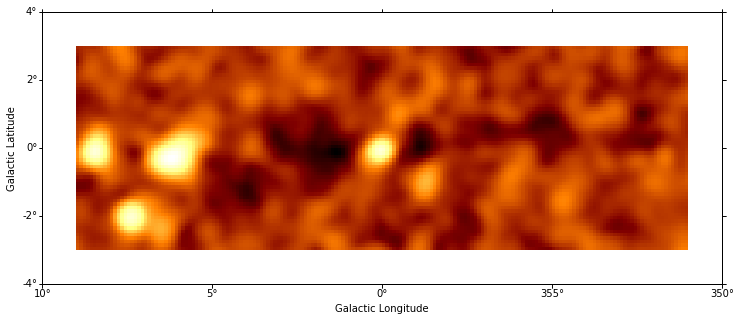
In [5]:

plt.figure(figsize=(15, 5))
images["sqrt_ts"].plot();

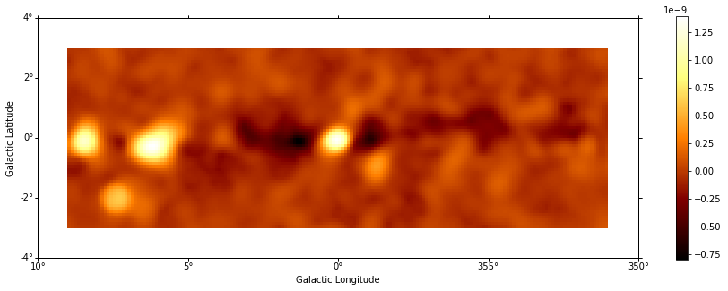
In [6]:

plt.figure(figsize=(15, 5))
images["flux"].plot(add_cbar=True);

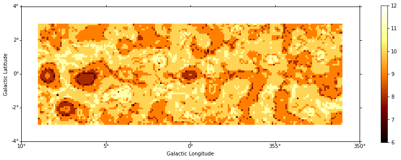
In [7]:

plt.figure(figsize=(15, 5))
images["niter"].plot(add_cbar=True);

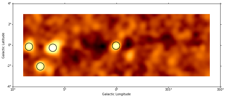
Source catalog¶

Let’s run a peak finder on the sqrt_ts image to get a list of sources (positions and peak sqrt_ts values).

In [8]:

sources = find_peaks(images["sqrt_ts"], threshold=8)
sources

Out[8]:

Table length=4

value	x	y	ra	dec
			deg	deg
float64	int64	int64	float64	float64
11.386	38	37	270.13528	-23.76653
10.044	15	38	271.27051	-21.71617
10.008	99	39	266.48351	-28.91953
9.7378	26	19	272.49049	-23.60089

In [9]:

# Plot sources on top of significance sky image
plt.figure(figsize=(15, 5))

images["sqrt_ts"].plot()

plt.gca().scatter(
    sources["ra"],
    sources["dec"],
    transform=plt.gca().get_transform("icrs"),
    color="none",
    edgecolor="black",
    marker="o",
    s=600,
    lw=1.5,
);

Measurements¶

TODO: show cutout for a few sources and some aperture photometry measurements (e.g. energy distribution, significance, flux)

In [10]:

# TODO

Compare to 2FHL¶

TODO

In [11]:

fermi_2fhl = source_catalogs["2fhl"]
fermi_2fhl.table[:5][["Source_Name", "GLON", "GLAT"]]

Out[11]:

Table length=5

Source_Name	GLON	GLAT
	deg	deg
bytes18	float32	float32
2FHL J0008.1+4709	115.339	-15.0688
2FHL J0009.3+5031	116.124	-11.7932
2FHL J0018.5+2947	114.463	-32.5424
2FHL J0022.0+0006	107.172	-61.8618
2FHL J0033.6-1921	94.28	-81.2224

Exercises¶

TODO: put one or more exercises

In [12]:

# Start exercises here!

What next?¶

In this notebook, we have seen how to work with images and compute TS images from counts data, if a background estimate is already available.

Here’s some suggestions what to do next:

TODO: point to background estimation examples
TODO: point to other docs …