This is a fixed-text formatted version of a Jupyter notebook.
- Try online

- You can contribute with your own notebooks in this GitHub repository.
- Source files: spectrum_pipe.ipynb | spectrum_pipe.py
Spectrum analysis with Gammapy (run pipeline)
In this tutorial we will learn how to perform a 1d spectral analysis.
We will use a “pipeline” or “workflow” class to run a standard analysis. If you’re interested in implementation detail of the analysis in order to create a custom analysis class, you should read (spectrum_analysis.ipynb) that executes the analysis using lower-level classes and methods in Gammapy.
In this tutorial we will use the folling Gammapy classes:
- gammapy.data.DataStore to load the data to
- gammapy.scripts.SpectrumAnalysisIACT to run the analysis
We use 4 Crab observations from H.E.S.S. for testing.
Setup
As usual, we’ll start with some setup for the notebook, and import the functionality we need.
In [1]:
%matplotlib inline
import numpy as np
import matplotlib.pyplot as plt

import astropy.units as u
from astropy.coordinates import SkyCoord
from regions import CircleSkyRegion

from gammapy.utils.energy import EnergyBounds
from gammapy.data import DataStore
from gammapy.scripts import SpectrumAnalysisIACT
from gammapy.catalog import SourceCatalogGammaCat
from gammapy.maps import Map
from gammapy.spectrum.models import LogParabola
from gammapy.spectrum import CrabSpectrum
Select data
First, we select and load some H.E.S.S. data (simulated events for now). In real life you would do something fancy here, or just use the list of observations someone send you (and hope they have done something fancy before). We’ll just use the standard gammapy 4 crab runs.
In [2]:
data_store = DataStore.from_dir("$GAMMAPY_DATA/hess-dl3-dr1/")
mask = data_store.obs_table["TARGET_NAME"] == "Crab"
obs_ids = data_store.obs_table["OBS_ID"][mask].data
observations = data_store.obs_list(obs_ids)
print(obs_ids)
[23523 23526 23559 23592]
Configure the analysis
Now we’ll define the input for the spectrum analysis. It will be done the python way, i.e. by creating a config dict containing python objects. We plan to add also the convenience to configure the analysis using a plain text config file.
In [3]:
crab_pos = SkyCoord.from_name("crab")
on_region = CircleSkyRegion(crab_pos, 0.15 * u.deg)

model = LogParabola(
    alpha=2.3,
    beta=0.01,
    amplitude=1e-11 * u.Unit("cm-2 s-1 TeV-1"),
    reference=1 * u.TeV,
)

flux_point_binning = EnergyBounds.equal_log_spacing(0.7, 30, 5, u.TeV)
In [4]:
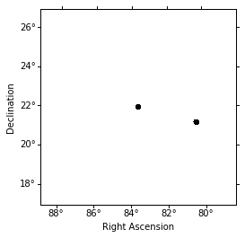
exclusion_mask = Map.create(skydir=crab_pos, width=(10, 10), binsz=0.02)

gammacat = SourceCatalogGammaCat()

regions = []
for source in gammacat:
    if not exclusion_mask.geom.contains(source.position):
        continue
    region = CircleSkyRegion(source.position, 0.15 * u.deg)
    regions.append(region)

exclusion_mask.data = exclusion_mask.geom.region_mask(regions, inside=False)
exclusion_mask.plot();
In [5]:
config = dict(
    outdir=".",
    background=dict(
        on_region=on_region,
        exclusion_mask=exclusion_mask,
        min_distance=0.1 * u.rad,
    ),
    extraction=dict(containment_correction=False),
    fit=dict(
        model=model,
        stat="wstat",
        forward_folded=True,
        fit_range=flux_point_binning[[0, -1]],
    ),
    fp_binning=flux_point_binning,
)
Run the analysis
TODO: Clean up the log (partly done, get rid of remaining useless warnings)
In [6]:
analysis = SpectrumAnalysisIACT(observations=observations, config=config)
analysis.run(optimize_opts={"print_level": 1})
| FCN = 108.83548502896386 | TOTAL NCALL = 118 | NCALLS = 118 |
| EDM = 2.6101091011340668e-06 | GOAL EDM = 1e-05 | UP = 1.0 |
| Valid | Valid Param | Accurate Covar | PosDef | Made PosDef |
| True | True | True | True | False |
| Hesse Fail | HasCov | Above EDM | Reach calllim | |
| False | True | False | False |
| + | Name | Value | Hesse Error | Minos Error- | Minos Error+ | Limit- | Limit+ | Fixed? |
| 0 | par_000_amplitude | 3.32931 | 0.222011 | No | ||||
| 1 | par_001_reference | 1 | 1 | Yes | ||||
| 2 | par_002_alpha | 2.32327 | 0.193054 | No | ||||
| 3 | par_003_beta | 18.6602 | 9.95332 | No |
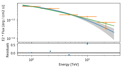
Results
Let’s look at the results, and also compare with a previously published Crab nebula spectrum for reference.
In [7]:
print(analysis.fit.result[0])
Fit result info
---------------
Model: LogParabola

Parameters:

           name     value     error         unit      min max
        --------- --------- --------- --------------- --- ---
        amplitude 3.329e-11 2.220e-12 1 / (cm2 s TeV) nan nan
        reference 1.000e+00 0.000e+00             TeV nan nan
            alpha 2.323e+00 1.931e-01                 nan nan
             beta 1.866e-01 9.953e-02                 nan nan

Covariance:

           name   amplitude  reference   alpha       beta
        --------- ---------- --------- ---------- ----------
        amplitude  4.929e-24 0.000e+00  2.248e-13 -6.322e-14
        reference  0.000e+00 0.000e+00  0.000e+00  0.000e+00
            alpha  2.248e-13 0.000e+00  3.727e-02 -1.744e-02
             beta -6.322e-14 0.000e+00 -1.744e-02  9.907e-03

Statistic: 39.258 (wstat)
Fit Range: [  0.87992254  27.82559402] TeV
In [8]:
opts = {
    "energy_range": analysis.fit.fit_range,
    "energy_power": 2,
    "flux_unit": "erg-1 cm-2 s-1",
}
axes = analysis.spectrum_result.plot(**opts)
CrabSpectrum().model.plot(ax=axes[0], **opts)
Out[8]:
<matplotlib.axes._subplots.AxesSubplot at 0x122981b00>
Exercises
Rerun the analysis, changing some aspects of the analysis as you like:
- only use one or two observations
- a different spectral model
- different config options for the spectral analysis
- different energy binning for the spectral point computation
Observe how the measured spectrum changes.