This is a fixed-text formatted version of a Jupyter notebook.
- Try online

- You can contribute with your own notebooks in this GitHub repository.
- Source files: sed_fitting_gammacat_fermi.ipynb | sed_fitting_gammacat_fermi.py
Flux point fitting in Gammapy
Introduction
In this tutorial we’re going to learn how to fit spectral models to combined Fermi-LAT and IACT flux points.
The central class we’re going to use for this example analysis is:
In addition we will work with the following data classes:
- gammapy.spectrum.FluxPoints
- gammapy.catalog.SourceCatalogGammaCat
- gammapy.catalog.SourceCatalog3FHL
- gammapy.catalog.SourceCatalog3FGL
And the following spectral model classes:
Setup
Let us start with the usual IPython notebook and Python imports:
In [1]:
%matplotlib inline
import numpy as np
import matplotlib.pyplot as plt
In [2]:
from astropy import units as u
from gammapy.spectrum.models import (
    PowerLaw,
    ExponentialCutoffPowerLaw,
    LogParabola,
)
from gammapy.spectrum import FluxPointFit, FluxPoints
from gammapy.catalog import (
    SourceCatalog3FGL,
    SourceCatalogGammaCat,
    SourceCatalog3FHL,
)
Load spectral points
For this analysis we choose to work with the source ‘HESS J1507-622’ and the associated Fermi-LAT sources ‘3FGL J1506.6-6219’ and ‘3FHL J1507.9-6228e’. We load the source catalogs, and then access source of interest by name:
In [3]:
fermi_3fgl = SourceCatalog3FGL()
fermi_3fhl = SourceCatalog3FHL()
gammacat = SourceCatalogGammaCat()
In [4]:
source_gammacat = gammacat["HESS J1507-622"]
source_fermi_3fgl = fermi_3fgl["3FGL J1506.6-6219"]
source_fermi_3fhl = fermi_3fhl["3FHL J1507.9-6228e"]
The corresponding flux points data can be accessed with .flux_points
attribute:
In [5]:
flux_points_gammacat = source_gammacat.flux_points
flux_points_gammacat.table
Out[5]:
| e_ref | dnde | dnde_errn | dnde_errp |
|---|---|---|---|
| TeV | 1 / (cm2 s TeV) | 1 / (cm2 s TeV) | 1 / (cm2 s TeV) |
| float32 | float32 | float32 | float32 |
| 0.8609 | 2.29119e-12 | 8.70543e-13 | 8.95502e-13 |
| 1.56151 | 6.98172e-13 | 2.20354e-13 | 2.30407e-13 |
| 2.76375 | 1.69062e-13 | 6.7587e-14 | 7.18838e-14 |
| 4.8916 | 7.72925e-14 | 2.40132e-14 | 2.60749e-14 |
| 9.98858 | 1.03253e-14 | 5.06315e-15 | 5.64195e-15 |
| 27.0403 | 7.44987e-16 | 5.72089e-16 | 7.25999e-16 |
In the Fermi-LAT catalogs, integral flux points are given. Currently the flux point fitter only works with differential flux points, so we apply the conversion here.
In [6]:
flux_points_3fgl = source_fermi_3fgl.flux_points.to_sed_type(
    sed_type="dnde", model=source_fermi_3fgl.spectral_model
)
flux_points_3fhl = source_fermi_3fhl.flux_points.to_sed_type(
    sed_type="dnde", model=source_fermi_3fhl.spectral_model
)
Finally we stack the flux points into a single FluxPoints object and
drop the upper limit values, because currently we can’t handle them in
the fit:
In [7]:
# stack flux point tables
flux_points = FluxPoints.stack(
    [flux_points_gammacat, flux_points_3fhl, flux_points_3fgl]
)

# drop the flux upper limit values
flux_points = flux_points.drop_ul()
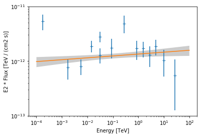
Power Law Fit
First we start with fitting a simple power law.
In [8]:
pwl = PowerLaw(index=2, amplitude="1e-12 cm-2 s-1 TeV-1", reference="1 TeV")
After creating the model we run the fit by passing the 'flux_points'
and 'pwl' objects:
In [9]:
fitter = FluxPointFit(pwl, flux_points, stat="chi2assym")
result_pwl = fitter.run()
And print the result:
In [10]:
print(result_pwl.model)
PowerLaw

Parameters:

           name     value     error         unit         min    max
        --------- --------- --------- --------------- --------- ---
            index 1.966e+00 2.651e-02                       nan nan
        amplitude 1.345e-12 1.595e-13 1 / (cm2 s TeV)       nan nan
        reference 1.000e+00 0.000e+00             TeV 0.000e+00 nan

Covariance:

           name     index    amplitude  reference
        --------- ---------- ---------- ---------
            index  7.029e-04 -2.230e-15 0.000e+00
        amplitude -2.230e-15  2.543e-26 0.000e+00
        reference  0.000e+00  0.000e+00 0.000e+00
Finally we plot the data points and the best fit model:
In [11]:
ax = flux_points.plot(energy_power=2)
result_pwl.model.plot(energy_range=[1e-4, 1e2] * u.TeV, ax=ax, energy_power=2)
result_pwl.model.plot_error(
    energy_range=[1e-4, 1e2] * u.TeV, ax=ax, energy_power=2
)
ax.set_ylim(1e-13, 1e-11);
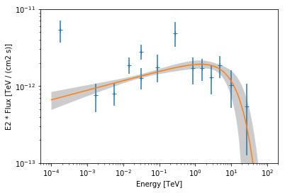
Exponential Cut-Off Powerlaw Fit
Next we fit an exponential cut-off power law to the data.
In [12]:
ecpl = ExponentialCutoffPowerLaw(
    index=2,
    amplitude="1e-12 cm-2 s-1 TeV-1",
    reference="1 TeV",
    lambda_="0.1 TeV-1",
)
We run the fitter again by passing the flux points and the ecpl
model instance:
In [13]:
fitter = FluxPointFit(ecpl, flux_points, stat="chi2assym")
result_ecpl = fitter.run()
print(result_ecpl.model)
ExponentialCutoffPowerLaw

Parameters:

           name     value     error         unit      min max
        --------- --------- --------- --------------- --- ---
            index 1.876e+00 4.517e-02                 nan nan
        amplitude 2.077e-12 4.105e-13 1 / (cm2 s TeV) nan nan
        reference 1.000e+00 0.000e+00             TeV nan nan
          lambda_ 8.703e-02 5.699e-02         1 / TeV nan nan

Covariance:

           name     index    amplitude  reference  lambda_
        --------- ---------- ---------- --------- ----------
            index  2.041e-03 -1.506e-14 0.000e+00 -1.832e-03
        amplitude -1.506e-14  1.685e-25 0.000e+00  1.851e-14
        reference  0.000e+00  0.000e+00 0.000e+00  0.000e+00
          lambda_ -1.832e-03  1.851e-14 0.000e+00  3.248e-03
We plot the data and best fit model:
In [14]:
ax = flux_points.plot(energy_power=2)
result_ecpl.model.plot(energy_range=[1e-4, 1e2] * u.TeV, ax=ax, energy_power=2)
result_ecpl.model.plot_error(
    energy_range=[1e-4, 1e2] * u.TeV, ax=ax, energy_power=2
)
ax.set_ylim(1e-13, 1e-11)
Out[14]:
(1e-13, 1e-11)
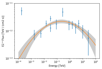
Log-Parabola Fit
Finally we try to fit a log-parabola model:
In [15]:
log_parabola = LogParabola(
    alpha=2, amplitude="1e-12 cm-2 s-1 TeV-1", reference="1 TeV", beta=0.1
)
In [16]:
fitter = FluxPointFit(log_parabola, flux_points, stat="chi2assym")
result_log_parabola = fitter.run()
print(result_log_parabola.model)
LogParabola

Parameters:

           name     value     error         unit      min max
        --------- --------- --------- --------------- --- ---
        amplitude 1.953e-12 2.799e-13 1 / (cm2 s TeV) nan nan
        reference 1.000e+00 0.000e+00             TeV nan nan
            alpha 2.161e+00 7.412e-02                 nan nan
             beta 5.385e-02 1.763e-02                 nan nan

Covariance:

           name   amplitude reference   alpha      beta
        --------- --------- --------- --------- ---------
        amplitude 7.835e-26 0.000e+00 1.753e-15 2.184e-15
        reference 0.000e+00 0.000e+00 0.000e+00 0.000e+00
            alpha 1.753e-15 0.000e+00 5.494e-03 1.127e-03
             beta 2.184e-15 0.000e+00 1.127e-03 3.109e-04
In [17]:
ax = flux_points.plot(energy_power=2)
result_log_parabola.model.plot(
    energy_range=[1e-4, 1e2] * u.TeV, ax=ax, energy_power=2
)
result_log_parabola.model.plot_error(
    energy_range=[1e-4, 1e2] * u.TeV, ax=ax, energy_power=2
)
ax.set_ylim(1e-13, 1e-11);
Exercises
- Fit a
PowerLaw2andExponentialCutoffPowerLaw3FGLto the same data. - Fit a
ExponentialCutoffPowerLawmodel to Vela X (‘HESS J0835-455’) only and check if the best fit values correspond to the values given in the Gammacat catalog
What next?
This was an introduction to SED fitting in Gammapy.
- If you would like to learn how to perform a full Poisson maximum likelihood spectral fit, please check out the spectrum pipe tutorial.
- If you are interested in simulation of spectral data in the context of CTA, please check out the spectrum simulation cta notebook.
- To learn more about other parts of Gammapy (e.g. Fermi-LAT and TeV data analysis), check out the other tutorial notebooks.
- To see what’s available in Gammapy, browse the Gammapy docs or use the full-text search.
- If you have any questions, ask on the mailing list .