This is a fixed-text formatted version of a Jupyter notebook.
- Try online

- You can contribute with your own notebooks in this GitHub repository.
- Source files: image_fitting_with_sherpa.ipynb | image_fitting_with_sherpa.py
Fitting 2D images with Sherpa
Introduction
Sherpa is the X-ray satellite Chandra modeling and fitting application. It enables the user to construct complex models from simple definitions and fit those models to data, using a variety of statistics and optimization methods. The issues of constraining the source position and morphology are common in X- and Gamma-ray astronomy. This notebook will show you how to apply Sherpa to CTA data.
Here we will set up Sherpa to fit the counts map and loading the ancillary images for subsequent use. A relevant test statistic for data with Poisson fluctuations is the one proposed by Cash (1979). The simplex (or Nelder-Mead) fitting algorithm is a good compromise between efficiency and robustness. The source fit is best performed in pixel coordinates.
Read sky images
The sky image that are loaded here have been prepared in a separated notebook. Here we start from those fits file and focus on the source fitting aspect.
The info needed for sherpa are: - Count map - Background map - Exposure map - PSF map
For info, the fits file are written in the following way in the Sky map generation notebook:
images['counts']    .write("G300-0_test_counts.fits", clobber=True)
images['exposure']  .write("G300-0_test_exposure.fits", clobber=True)
images['background'].write("G300-0_test_background.fits", clobber=True)

##As psf is an array of quantities we cannot use the images['psf'].write() function
##all the other arrays do not have quantities.
fits.writeto("G300-0_test_psf.fits",images['psf'].data.value,overwrite=True)
In [1]:
%matplotlib inline
import matplotlib.pyplot as plt
import numpy as np
from astropy.coordinates import SkyCoord
import astropy.units as u
from astropy.io import fits
from astropy.wcs import WCS
from gammapy.maps import Map, WcsNDMap, WcsGeom
import os

# Warnings about XSPEC or DS9 can be ignored here
import sherpa.astro.ui as sh
WARNING: imaging routines will not be available,
failed to import sherpa.image.ds9_backend due to
'RuntimeErr: DS9Win unusable: Could not find ds9 on your PATH'
WARNING: failed to import sherpa.astro.xspec; XSPEC models will not be available
In [2]:
# Read the fits file to load them in a sherpa model
filecounts = os.environ["GAMMAPY_DATA"] + "/sherpaCTA/G300-0_test_counts.fits"
hdr = fits.getheader(filecounts)
wcs = WCS(hdr)

sh.set_stat("cash")
sh.set_method("simplex")
sh.load_image(filecounts)
sh.set_coord("logical")

fileexp = os.environ["GAMMAPY_DATA"] + "/sherpaCTA/G300-0_test_exposure.fits"
filebkg = os.environ["GAMMAPY_DATA"] + "/sherpaCTA/G300-0_test_background.fits"
filepsf = os.environ["GAMMAPY_DATA"] + "/sherpaCTA/G300-0_test_psf.fits"
sh.load_table_model("expo", fileexp)
sh.load_table_model("bkg", filebkg)
sh.load_psf("psf", filepsf)
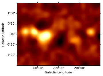
In principle one might first want to fit the background amplitude. However the background estimation method already yields the correct normalization, so we freeze the background amplitude to unity instead of adjusting it. The (smoothed) residuals from this background model are then computed and shown.
In [3]:
sh.set_full_model(bkg)
bkg.ampl = 1
sh.freeze(bkg)

resid = Map.read(filecounts)
resid.data = sh.get_data_image().y - sh.get_model_image().y
resid_smooth = resid.smooth(width=6)
resid_smooth.plot();
Find and fit the brightest source
We then find the position of the maximum in the (smoothed) residuals map, and fit a (symmetrical) Gaussian source with that initial position:
In [4]:
yp, xp = np.unravel_index(
    np.nanargmax(resid_smooth.data), resid_smooth.data.shape
)
ampl = resid_smooth.get_by_pix((xp, yp))[0]

sh.set_full_model(
    bkg + psf(sh.gauss2d.g0) * expo
)  # creates g0 as a gauss2d instance
g0.xpos, g0.ypos = xp, yp
sh.freeze(g0.xpos, g0.ypos)  # fix the position in the initial fitting step

expo.ampl = (
    1e-9
)  # fix exposure amplitude so that typical exposure is of order unity
sh.freeze(expo)
sh.thaw(g0.fwhm, g0.ampl)  # in case frozen in a previous iteration

g0.fwhm = 10  # give some reasonable initial values
g0.ampl = ampl
In [5]:
%%time
sh.fit()
Dataset               = 1
Method                = neldermead
Statistic             = cash
Initial fit statistic = 47566.1
Final fit statistic   = 47440.7 at function evaluation 228
Data points           = 30000
Degrees of freedom    = 29998
Change in statistic   = 125.402
   g0.fwhm        20.0951
   g0.ampl        0.111272
CPU times: user 1.58 s, sys: 17 ms, total: 1.6 s
Wall time: 1.62 s
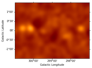
Fit all parameters of this Gaussian component, fix them and re-compute the residuals map.
In [6]:
sh.thaw(g0.xpos, g0.ypos)
sh.fit()
sh.freeze(g0)

resid.data = sh.get_data_image().y - sh.get_model_image().y
resid_smooth = resid.smooth(width=6)
resid_smooth.plot(vmin=-0.5, vmax=1);
Dataset               = 1
Method                = neldermead
Statistic             = cash
Initial fit statistic = 47440.7
Final fit statistic   = 47429.2 at function evaluation 408
Data points           = 30000
Degrees of freedom    = 29996
Change in statistic   = 11.4937
   g0.fwhm        21.5373
   g0.xpos        66.3947
   g0.ypos        69.3172
   g0.ampl        0.107149
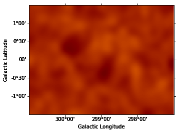
Iteratively find and fit additional sources
Instantiate additional Gaussian components, and use them to iteratively fit sources, repeating the steps performed above for component g0. (The residuals map is shown after each additional source included in the model.) This takes some time…
In [7]:
# initialize components with fixed, zero amplitude
for i in range(1, 6):
    model = sh.create_model_component("gauss2d", "g" + str(i))
    model.ampl = 0
    sh.freeze(model)

gs = [g0, g1, g2, g3, g4, g5]
sh.set_full_model(bkg + psf(g0 + g1 + g2 + g3 + g4 + g5) * expo)
In [8]:
%%time
for i in range(1, len(gs)):
    yp, xp = np.unravel_index(
        np.nanargmax(resid_smooth.data), resid_smooth.data.shape
    )
    ampl = resid_smooth.get_by_pix((xp, yp))[0]
    gs[i].xpos, gs[i].ypos = xp, yp
    gs[i].fwhm = 10
    gs[i].ampl = ampl

    sh.thaw(gs[i].fwhm)
    sh.thaw(gs[i].ampl)
    sh.fit()

    sh.thaw(gs[i].xpos)
    sh.thaw(gs[i].ypos)
    sh.fit()
    sh.freeze(gs[i])

    resid.data = sh.get_data_image().y - sh.get_model_image().y
    resid_smooth = resid.smooth(width=6)
    resid_smooth.plot(vmin=-0.5, vmax=1)
Dataset               = 1
Method                = neldermead
Statistic             = cash
Initial fit statistic = 47352.1
Final fit statistic   = 47306.6 at function evaluation 218
Data points           = 30000
Degrees of freedom    = 29998
Change in statistic   = 45.4492
   g1.fwhm        6.73141
   g1.ampl        0.358694
Dataset               = 1
Method                = neldermead
Statistic             = cash
Initial fit statistic = 47306.6
Final fit statistic   = 47295.3 at function evaluation 362
Data points           = 30000
Degrees of freedom    = 29996
Change in statistic   = 11.3247
   g1.fwhm        5.88307
   g1.xpos        41.7803
   g1.ypos        81.4247
   g1.ampl        0.45753
Dataset               = 1
Method                = neldermead
Statistic             = cash
Initial fit statistic = 47211.4
Final fit statistic   = 47187.6 at function evaluation 215
Data points           = 30000
Degrees of freedom    = 29998
Change in statistic   = 23.794
   g2.fwhm        6.77442
   g2.ampl        0.346582
Dataset               = 1
Method                = neldermead
Statistic             = cash
Initial fit statistic = 47187.6
Final fit statistic   = 47184.1 at function evaluation 341
Data points           = 30000
Degrees of freedom    = 29996
Change in statistic   = 3.46844
   g2.fwhm        6.19417
   g2.xpos        20.8277
   g2.ypos        81.6412
   g2.ampl        0.399908
Dataset               = 1
Method                = neldermead
Statistic             = cash
Initial fit statistic = 47173.4
Final fit statistic   = 47116.6 at function evaluation 227
Data points           = 30000
Degrees of freedom    = 29998
Change in statistic   = 56.7946
   g3.fwhm        6.43218
   g3.ampl        0.235481
Dataset               = 1
Method                = neldermead
Statistic             = cash
Initial fit statistic = 47116.6
Final fit statistic   = 47115.9 at function evaluation 303
Data points           = 30000
Degrees of freedom    = 29996
Change in statistic   = 0.728928
   g3.fwhm        6.38175
   g3.xpos        177.458
   g3.ypos        80.2233
   g3.ampl        0.239637
Dataset               = 1
Method                = neldermead
Statistic             = cash
Initial fit statistic = 47121
Final fit statistic   = 47090.2 at function evaluation 246
Data points           = 30000
Degrees of freedom    = 29998
Change in statistic   = 30.818
   g4.fwhm        7.24022
   g4.ampl        0.112126
Dataset               = 1
Method                = neldermead
Statistic             = cash
Initial fit statistic = 47090.2
Final fit statistic   = 47087.3 at function evaluation 330
Data points           = 30000
Degrees of freedom    = 29996
Change in statistic   = 2.93503
   g4.fwhm        5.94179
   g4.xpos        135.942
   g4.ypos        59.5875
   g4.ampl        0.156213
Dataset               = 1
Method                = neldermead
Statistic             = cash
Initial fit statistic = 47082.3
Final fit statistic   = 47068.5 at function evaluation 249
Data points           = 30000
Degrees of freedom    = 29998
Change in statistic   = 13.7724
   g5.fwhm        3.07232
   g5.ampl        0.479624
Dataset               = 1
Method                = neldermead
Statistic             = cash
Initial fit statistic = 47068.5
Final fit statistic   = 47068.5 at function evaluation 320
Data points           = 30000
Degrees of freedom    = 29996
Change in statistic   = 0.0196613
   g5.fwhm        3.05445
   g5.xpos        76.0488
   g5.ypos        73.1002
   g5.ampl        0.483818
CPU times: user 25.7 s, sys: 267 ms, total: 26 s
Wall time: 26.3 s
Generating output table and Test Statistics estimation
When adding a new source, one need to check the significance of this new source. A frequently used method is the Test Statistics (TS). This is done by comparing the change of statistics when the source is included compared to the null hypothesis (no source ; in practice here we fix the amplitude to zero).
\(TS = Cstat(source) - Cstat(no source)\)
The criterion for a significant source detection is typically that it should improve the test statistic by at least 25 or 30. The last excess fitted (g5) thus not a significant source:
In [9]:
from astropy.stats import gaussian_fwhm_to_sigma
from astropy.table import Table

rows = []
for g in gs:
    ampl = g.ampl.val
    g.ampl = 0
    stati = sh.get_stat_info()[0].statval
    g.ampl = ampl
    statf = sh.get_stat_info()[0].statval
    delstat = stati - statf

    geom = resid.geom
    coord = geom.pix_to_coord((g.xpos.val, g.ypos.val))
    pix_scale = geom.pixel_scales.mean().deg
    sigma = g.fwhm.val * pix_scale * gaussian_fwhm_to_sigma
    rows.append(
        dict(delstat=delstat, glon=coord[0], glat=coord[1], sigma=sigma)
    )

table = Table(rows=rows, names=rows[0])
for name in table.colnames:
    table[name].format = ".5g"
table
Out[9]:
| delstat | glon | glat | sigma |
|---|---|---|---|
| float64 | float64 | float64 | float64 |
| 156.52 | 299.66 | -0.10365 | 0.18292 |
| 133.86 | 300.15 | 0.13847 | 0.049966 |
| 111.18 | 300.57 | 0.14277 | 0.052608 |
| 68.202 | 297.44 | 0.11442 | 0.054202 |
| 28.633 | 298.27 | -0.29822 | 0.050465 |
| 18.816 | 299.47 | -0.027994 | 0.025942 |
Exercises
- If you look back to the original image: there’s one source that looks
like a shell-type supernova remnant.
- Try to fit is with a shell morphology model (use
sh.shell2d('shell')to create such a model). - Try to evaluate the
TSand probability of the shell model compared to a Gaussian model hypothesis - You could also try a disk model (use
sh.disk2d('disk')to create one)
- Try to fit is with a shell morphology model (use
What next?
These are good resources to learn more about Sherpa:
- https://python4astronomers.github.io/fitting/fitting.html
- https://github.com/DougBurke/sherpa-standalone-notebooks
You could read over the examples there, and try to apply a similar analysis to this dataset here to practice.
If you want a deeper understanding of how Sherpa works, then these proceedings are good introductions: