This is a fixed-text formatted version of a Jupyter notebook.
- Try online

- You can contribute with your own notebooks in this GitHub repository.
- Source files: hess.ipynb | hess.py
H.E.S.S. with Gammapy
This tutorial explains how to analyse H.E.S.S. data with Gammapy.
We will analyse four observation runs of the Crab nebula, which are part of the H.E.S.S. first public test data release. In this tutorial we will make an image and a spectrum. The light_curve.ipynb notbook contains an example how to make a light curve.
To do a 3D analysis, one needs to do a 3D background estimate. In background_model.ipynb we have started to make a background model, and in this notebook we have a first look at a 3D analysis. But the results aren’t OK yet, the background model needs to be improved. In this analysis, we also don’t use the energy dispersion IRF yet, and we only analyse the data in the 1 TeV to 10 TeV range. The H.E.S.S. data was only released very recently, and 3D analysis in Gammapy is new. This tutorial will be improved soon.
In [1]:
%matplotlib inline
import matplotlib.pyplot as plt
In [2]:
import numpy as np
import astropy.units as u
from astropy.coordinates import SkyCoord
from regions import CircleSkyRegion
from gammapy.data import DataStore
from gammapy.maps import Map, MapAxis, WcsGeom, WcsNDMap
from gammapy.cube import MapMaker, MapFit, PSFKernel
from gammapy.cube.models import SkyModel
from gammapy.spectrum.models import PowerLaw, ExponentialCutoffPowerLaw
from gammapy.image.models import SkyGaussian, SkyPointSource
from gammapy.detect import TSMapEstimator
from gammapy.scripts import SpectrumAnalysisIACT
Data access
To access the data, we use the DataStore, and we use the
obs_table to select the Crab runs.
In [3]:
data_store = DataStore.from_file(
    "$GAMMAPY_DATA/hess-dl3-dr1/hess-dl3-dr3-with-background.fits.gz"
)
mask = data_store.obs_table["TARGET_NAME"] == "Crab"
obs_table = data_store.obs_table[mask]
observations = data_store.obs_list(obs_table["OBS_ID"])
In [4]:
# pos_crab = SkyCoord.from_name('Crab')
pos_crab = SkyCoord(83.633, 22.014, unit="deg")
Maps
Let’s make some 3D cubes, as well as 2D images.
For the energy, we make 5 bins from 1 TeV to 10 TeV.
In [5]:
energy_axis = MapAxis.from_edges(
    np.logspace(0, 1., 5), unit="TeV", name="energy", interp="log"
)
geom = WcsGeom.create(
    skydir=(83.633, 22.014),
    binsz=0.02,
    width=(5, 5),
    coordsys="CEL",
    proj="TAN",
    axes=[energy_axis],
)
In [6]:
%%time
maker = MapMaker(geom, offset_max="2.5 deg")
maps = maker.run(observations)
images = maker.make_images()
CPU times: user 3.76 s, sys: 444 ms, total: 4.2 s
Wall time: 4.26 s
In [7]:
maps.keys()
Out[7]:
dict_keys(['counts', 'exposure', 'background'])
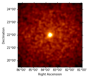
In [8]:
images["counts"].smooth(3).plot(stretch="sqrt", vmax=2);
PSF
Compute the mean PSF for these observations at the Crab position.
In [9]:
table_psf = observations.make_mean_psf(pos_crab)
/Users/jer/anaconda/envs/gammapy-dev/lib/python3.6/site-packages/astropy/units/quantity.py:639: RuntimeWarning: invalid value encountered in true_divide
  result = super().__array_ufunc__(function, method, *arrays, **kwargs)
In [10]:
psf_kernel = PSFKernel.from_table_psf(table_psf, geom, max_radius="0.3 deg")
psf_kernel_array = psf_kernel.psf_kernel_map.sum_over_axes().data
# psf_kernel.psf_kernel_map.slice_by_idx({'energy': 0}).plot()
# plt.imshow(psf_kernel_array)
Map fit
Let’s fit this source assuming a Gaussian spatial shape and a power-law spectral shape
In [11]:
spatial_model = SkyPointSource(lon_0="83.6 deg", lat_0="22.0 deg")
spectral_model = PowerLaw(
    index=2.6, amplitude="5e-11 cm-2 s-1 TeV-1", reference="1 TeV"
)
model = SkyModel(spatial_model=spatial_model, spectral_model=spectral_model)
In [12]:
%%time
fit = MapFit(
    model=model,
    counts=maps["counts"],
    exposure=maps["exposure"],
    background=maps["background"],
    psf=psf_kernel,
)
result = fit.run()
print(result)
print(result.model.parameters.to_table())
FitResult

        backend    : minuit
        method     : minuit
        success    : True
        nfev       : 108
        total stat : 66212.33
        message    : Optimization terminated successfully.

   name     value     error         unit         min    max
--------- --------- --------- --------------- --------- ---
    lon_0 8.362e+01 2.730e-03             deg       nan nan
    lat_0 2.203e+01 2.468e-03             deg       nan nan
    index 2.617e+00 8.196e-02                       nan nan
amplitude 5.923e-11 4.370e-12 1 / (cm2 s TeV)       nan nan
reference 1.000e+00 0.000e+00             TeV 0.000e+00 nan
CPU times: user 4.19 s, sys: 119 ms, total: 4.3 s
Wall time: 4.56 s
Residual image
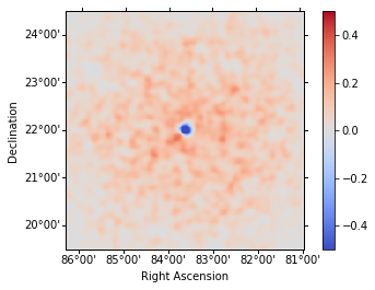
We compute a residual image as residual = counts - model. Note that
this is counts per pixel and our pixel size is 0.02 deg. Smoothing is
counts-preserving. The residual image shows that currently both the
source and the background modeling isn’t very good. The background model
is underestimated (so residual is positive), and the source model is
overestimated.
In [13]:
npred = fit.evaluator.compute_npred()
residual = Map.from_geom(maps["counts"].geom)
residual.data = maps["counts"].data - npred.data
In [14]:
residual.sum_over_axes().smooth(3).plot(
    cmap="coolwarm", vmin=-0.5, vmax=0.5, add_cbar=True
);
Spectrum
We could try to improve the background modeling and spatial model of the source. But let’s instead turn to one of the classic IACT analysis techniques: use a circular on region and reflected regions for background estimation, and derive a spectrum for the source without having to assume a spatial model, or without needing a 3D background model.
In [15]:
%%time
on_region = CircleSkyRegion(pos_crab, 0.11 * u.deg)
exclusion_mask = images["counts"].copy()
exclusion_mask.data = np.ones_like(exclusion_mask.data, dtype=bool)

model = PowerLaw(
    index=2.6, amplitude="5e-11 cm-2 s-1 TeV-1", reference="1 TeV"
)

config = {
    "outdir": ".",
    "background": {"on_region": on_region, "exclusion_mask": exclusion_mask},
    "extraction": {"containment_correction": True},
    "fit": {"model": model, "fit_range": [1, 10] * u.TeV},
    "fp_binning": np.logspace(0, 1, 7) * u.TeV,
}
analysis = SpectrumAnalysisIACT(observations=observations, config=config)
analysis.run()
CPU times: user 7.51 s, sys: 72.2 ms, total: 7.58 s
Wall time: 7.69 s
In [16]:
print(analysis.fit.result[0])
Fit result info
---------------
Model: PowerLaw

Parameters:

           name     value     error         unit         min    max
        --------- --------- --------- --------------- --------- ---
            index 2.577e+00 1.078e-01                       nan nan
        amplitude 4.354e-11 3.959e-12 1 / (cm2 s TeV)       nan nan
        reference 1.000e+00 0.000e+00             TeV 0.000e+00 nan

Covariance:

           name     index   amplitude reference
        --------- --------- --------- ---------
            index 1.163e-02 3.288e-13 0.000e+00
        amplitude 3.288e-13 1.567e-23 0.000e+00
        reference 0.000e+00 0.000e+00 0.000e+00

Statistic: 27.477 (wstat)
Fit Range: [  1.  10.] TeV
In [17]:
opts = {
    "energy_range": analysis.fit.fit_range,
    "energy_power": 2,
    "flux_unit": "erg-1 cm-2 s-1",
}
axes = analysis.spectrum_result.plot(**opts)
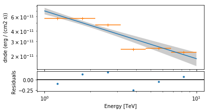
Again: please note that this tutorial notebook was put together quickly, the results obtained here are very preliminary. We will work on Gammapy and the analysis of data from the H.E.S.S. test release and update this tutorial soon.
Exercises
- Try analysing another source, e.g. MSH 15-52.
- Try another model, e.g. a Gaussian spatial shape or exponential cutoff power-law spectrum.