This is a fixed-text formatted version of a Jupyter notebook.
- Try online

- You can contribute with your own notebooks in this GitHub repository.
- Source files: spectrum_models.ipynb | spectrum_models.py
Spectral models in Gammapy
Introduction
This notebook explains how to use the functions and classes in gammapy.spectrum.models in order to work with spectral models.
The following clases will be used:
Setup
Same procedure as in every script …
In [1]:
%matplotlib inline
import matplotlib.pyplot as plt
In [2]:
import numpy as np
import astropy.units as u
from gammapy.spectrum import models
from gammapy.utils.fitting import Parameter, Parameters
Create a model
To create a spectral model, instantiate an object of the spectral model class you’re interested in.
In [3]:
pwl = models.PowerLaw()
print(pwl)
PowerLaw

Parameters:

           name     value   error       unit         min    max
        --------- --------- ----- --------------- --------- ---
            index 2.000e+00   nan                       nan nan
        amplitude 1.000e-12   nan 1 / (cm2 s TeV)       nan nan
        reference 1.000e+00   nan             TeV 0.000e+00 nan
This will use default values for the model parameters, which is rarely what you want.
Usually you will want to specify the parameters on object creation. One
way to do this is to pass astropy.utils.Quantity objects like this:
In [4]:
pwl = models.PowerLaw(
    index=2.3, amplitude=1e-12 * u.Unit("cm-2 s-1 TeV-1"), reference=1 * u.TeV
)
print(pwl)
PowerLaw

Parameters:

           name     value   error       unit         min    max
        --------- --------- ----- --------------- --------- ---
            index 2.300e+00   nan                       nan nan
        amplitude 1.000e-12   nan 1 / (cm2 s TeV)       nan nan
        reference 1.000e+00   nan             TeV 0.000e+00 nan
As you see, some of the parameters have default min and values
as well as a frozen flag. This is only relevant in the context of
spectral fitting and thus covered in
spectrum_analysis.ipynb.
Also, the parameter errors are not set. This will be covered later in
this tutorial.
Get and set model parameters
The model parameters are stored in the Parameters object on the
spectal model. Each model parameter is a Parameter instance. It has
a value and a unit attribute, as well as a quantity property
for convenience.
In [5]:
print(pwl.parameters)
Parameters
Parameter(name='index', value=2.3, factor=2.3, scale=1, unit='', min=nan, max=nan, frozen=False)
Parameter(name='amplitude', value=1e-12, factor=1e-12, scale=1, unit='cm-2 s-1 TeV-1', min=nan, max=nan, frozen=False)
Parameter(name='reference', value=1.0, factor=1.0, scale=1, unit='TeV', min=0.0, max=nan, frozen=True)

Covariance:
None
In [6]:
print(pwl.parameters["index"])
pwl.parameters["index"].value = 2.6
print(pwl.parameters["index"])
Parameter(name='index', value=2.3, factor=2.3, scale=1, unit='', min=nan, max=nan, frozen=False)
Parameter(name='index', value=2.6, factor=2.6, scale=1, unit='', min=nan, max=nan, frozen=False)
In [7]:
print(pwl.parameters["amplitude"])
pwl.parameters["amplitude"].quantity = 2e-12 * u.Unit("m-2 TeV-1 s-1")
print(pwl.parameters["amplitude"])
Parameter(name='amplitude', value=1e-12, factor=1e-12, scale=1, unit='cm-2 s-1 TeV-1', min=nan, max=nan, frozen=False)
Parameter(name='amplitude', value=2e-12, factor=2e-12, scale=1, unit='m-2 s-1 TeV-1', min=nan, max=nan, frozen=False)
List available models
All spectral models in gammapy are subclasses of SpectralModel. The
list of available models is shown below.
In [8]:
models.SpectralModel.__subclasses__()
Out[8]:
[gammapy.spectrum.models.ConstantModel,
 gammapy.spectrum.models.CompoundSpectralModel,
 gammapy.spectrum.models.PowerLaw,
 gammapy.spectrum.models.PowerLaw2,
 gammapy.spectrum.models.ExponentialCutoffPowerLaw,
 gammapy.spectrum.models.ExponentialCutoffPowerLaw3FGL,
 gammapy.spectrum.models.PLSuperExpCutoff3FGL,
 gammapy.spectrum.models.LogParabola,
 gammapy.spectrum.models.TableModel,
 gammapy.spectrum.models.AbsorbedSpectralModel,
 gammapy.spectrum.crab.MeyerCrabModel]
Plotting
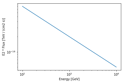
In order to plot a model you can use the plot function. It expects
an energy range as argument. You can also chose flux and energy units as
well as an energy power for the plot
In [9]:
energy_range = [0.1, 10] * u.TeV
pwl.plot(energy_range, energy_power=2, energy_unit="GeV")
Out[9]:
<matplotlib.axes._subplots.AxesSubplot at 0x115697550>
Parameter errors
Parameters are stored internally as covariance matrix. There are, however, convenience methods to set individual parameter errors.
In [10]:
pwl.parameters.set_parameter_errors(
    {"index": 0.2, "amplitude": 0.1 * pwl.parameters["amplitude"].quantity}
)
print(pwl)
PowerLaw

Parameters:

           name     value     error        unit         min    max
        --------- --------- --------- -------------- --------- ---
            index 2.600e+00 2.000e-01                      nan nan
        amplitude 2.000e-12 2.000e-13 1 / (m2 s TeV)       nan nan
        reference 1.000e+00 0.000e+00            TeV 0.000e+00 nan

Covariance:

           name     index   amplitude reference
        --------- --------- --------- ---------
            index 4.000e-02 0.000e+00 0.000e+00
        amplitude 0.000e+00 4.000e-26 0.000e+00
        reference 0.000e+00 0.000e+00 0.000e+00
You can access the parameter errors like this
In [11]:
pwl.parameters.covariance
Out[11]:
array([[  4.00000000e-02,   0.00000000e+00,   0.00000000e+00],
       [  0.00000000e+00,   4.00000000e-26,   0.00000000e+00],
       [  0.00000000e+00,   0.00000000e+00,   0.00000000e+00]])
In [12]:
pwl.parameters.error("index")
Out[12]:
0.20000000000000001
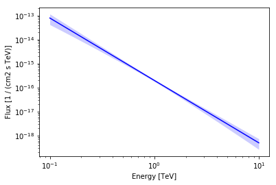
You can plot the butterfly using the plot_error method.
In [13]:
ax = pwl.plot_error(energy_range, color="blue", alpha=0.2)
pwl.plot(energy_range, ax=ax, color="blue");
Integral fluxes
You’ve probably asked yourself already, if it’s possible to integrated models. Yes, it is. Where analytical solutions are available, these are used by default. Otherwise, a numerical integration is performed.
In [14]:
pwl.integral(emin=1 * u.TeV, emax=10 * u.TeV)
Out[14]:
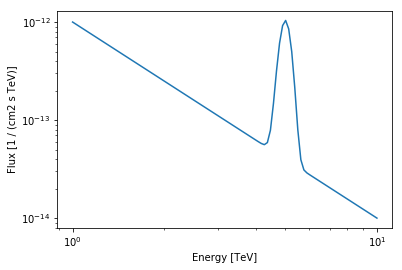
User-defined model
Now we’ll see how you can define a custom model. To do that you need to
subclass SpectralModel. All SpectralModel subclasses need to
have an __init__ function, which sets up the Parameters of the
model and a static function called evaluate where the
mathematical expression for the model is defined.
As an example we will use a PowerLaw plus a Gaussian (with fixed width).
In [15]:
class UserModel(models.SpectralModel):
    def __init__(self, index, amplitude, reference, mean, width):
        self.parameters = Parameters(
            [
                Parameter("index", index, min=0),
                Parameter("amplitude", amplitude, min=0),
                Parameter("reference", reference, frozen=True),
                Parameter("mean", mean, min=0),
                Parameter("width", width, min=0, frozen=True),
            ]
        )

    @staticmethod
    def evaluate(energy, index, amplitude, reference, mean, width):
        pwl = models.PowerLaw.evaluate(
            energy=energy,
            index=index,
            amplitude=amplitude,
            reference=reference,
        )
        gauss = amplitude * np.exp(-(energy - mean) ** 2 / (2 * width ** 2))
        return pwl + gauss
In [16]:
model = UserModel(
    index=2,
    amplitude=1e-12 * u.Unit("cm-2 s-1 TeV-1"),
    reference=1 * u.TeV,
    mean=5 * u.TeV,
    width=0.2 * u.TeV,
)
print(model)
UserModel

Parameters:

           name     value   error       unit         min    max
        --------- --------- ----- --------------- --------- ---
            index 2.000e+00   nan                 0.000e+00 nan
        amplitude 1.000e-12   nan 1 / (cm2 s TeV) 0.000e+00 nan
        reference 1.000e+00   nan             TeV       nan nan
             mean 5.000e+00   nan             TeV 0.000e+00 nan
            width 2.000e-01   nan             TeV 0.000e+00 nan
In [17]:
energy_range = [1, 10] * u.TeV
model.plot(energy_range=energy_range);
What’s next?
In this tutorial we learnd how to work with spectral models.
Go to gammapy.spectrum to learn more.