This is a fixed-text formatted version of a Jupyter notebook.
- Try online

- You can contribute with your own notebooks in this GitHub repository.
- Source files: simulate_3d.ipynb | simulate_3d.py
3D simulation and fitting
This tutorial shows how to do a 3D map-based simulation and fit.
For a tutorial on how to do a 3D map analyse of existing data, see the
analysis_3d tutorial.
This can be useful to do a performance / sensitivity study, or to evaluate the capabilities of Gammapy or a given analysis method. Note that is is a binned simulation as is e.g. done also in Sherpa for Chandra, not an event sampling and anbinned analysis as is done e.g. in the Fermi ST or ctools.
Imports and versions
In [1]:
%matplotlib inline
import matplotlib.pyplot as plt
In [2]:
import numpy as np
import astropy.units as u
from astropy.coordinates import SkyCoord, Angle
from gammapy.irf import (
    EffectiveAreaTable2D,
    EnergyDispersion2D,
    EnergyDependentMultiGaussPSF,
    Background3D,
)
from gammapy.maps import WcsGeom, MapAxis, WcsNDMap, Map
from gammapy.spectrum.models import PowerLaw
from gammapy.image.models import SkyGaussian
from gammapy.cube.models import SkyModel, SkyModels
from gammapy.cube import MapFit, MapEvaluator, PSFKernel
from gammapy.cube import make_map_exposure_true_energy, make_map_background_irf
In [3]:
!gammapy info --no-envvar --no-dependencies --no-system
Gammapy package:

        path                   : /Users/jer/git/gammapy/gammapy
        version                : 0.8
Simulate
In [4]:
def get_irfs():
    """Load CTA IRFs"""
    filename = "$GAMMAPY_DATA/cta-1dc/caldb/data/cta/1dc/bcf/South_z20_50h/irf_file.fits"
    psf = EnergyDependentMultiGaussPSF.read(
        filename, hdu="POINT SPREAD FUNCTION"
    )
    aeff = EffectiveAreaTable2D.read(filename, hdu="EFFECTIVE AREA")
    edisp = EnergyDispersion2D.read(filename, hdu="ENERGY DISPERSION")
    bkg = Background3D.read(filename, hdu="BACKGROUND")
    return dict(psf=psf, aeff=aeff, edisp=edisp, bkg=bkg)


irfs = get_irfs()
In [5]:
# Define sky model to simulate the data
spatial_model = SkyGaussian(lon_0="0.2 deg", lat_0="0.1 deg", sigma="0.3 deg")
spectral_model = PowerLaw(
    index=3, amplitude="1e-11 cm-2 s-1 TeV-1", reference="1 TeV"
)
sky_model = SkyModel(
    spatial_model=spatial_model, spectral_model=spectral_model
)
print(sky_model)
SkyModel

spatial_model = SkyGaussian

Parameters:

         name   value   error unit min max
        ----- --------- ----- ---- --- ---
        lon_0 2.000e-01   nan  deg nan nan
        lat_0 1.000e-01   nan  deg nan nan
        sigma 3.000e-01   nan  deg nan nan

spectral_model = PowerLaw

Parameters:

           name     value   error       unit         min    max
        --------- --------- ----- --------------- --------- ---
            index 3.000e+00   nan                       nan nan
        amplitude 1.000e-11   nan 1 / (cm2 s TeV)       nan nan
        reference 1.000e+00   nan             TeV 0.000e+00 nan
In [6]:
# Define map geometry
axis = MapAxis.from_edges(
    np.logspace(-1., 1., 10), unit="TeV", name="energy", interp="log"
)
geom = WcsGeom.create(
    skydir=(0, 0), binsz=0.02, width=(5, 4), coordsys="GAL", axes=[axis]
)
In [7]:
# Define some observation parameters
# Here we just have a single observation,
# we are not simulating many pointings / observations
pointing = SkyCoord(1, 0.5, unit="deg", frame="galactic")
livetime = 1 * u.hour
offset_max = 2 * u.deg
offset = Angle("2 deg")
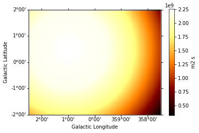
In [8]:
exposure = make_map_exposure_true_energy(
    pointing=pointing, livetime=livetime, aeff=irfs["aeff"], geom=geom
)
exposure.slice_by_idx({"energy": 3}).plot(add_cbar=True);
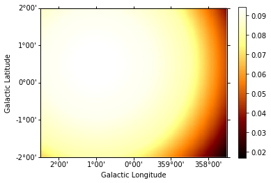
In [9]:
background = make_map_background_irf(
    pointing=pointing, livetime=livetime, bkg=irfs["bkg"], geom=geom
)
background.slice_by_idx({"energy": 3}).plot(add_cbar=True);
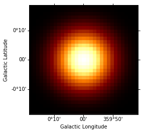
In [10]:
psf = irfs["psf"].to_energy_dependent_table_psf(theta=offset)
psf_kernel = PSFKernel.from_table_psf(psf, geom, max_radius=0.3 * u.deg)
psf_kernel.psf_kernel_map.sum_over_axes().plot(stretch="log");
In [11]:
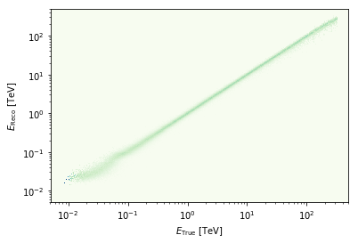
edisp = irfs["edisp"].to_energy_dispersion(offset=offset)
edisp.plot_matrix();
In [12]:
%%time
# The idea is that we have this class that can compute `npred`
# maps, i.e. "predicted counts per pixel" given the model and
# the observation infos: exposure, background, PSF and EDISP
evaluator = MapEvaluator(
    model=sky_model, exposure=exposure, background=background, psf=psf_kernel
)
CPU times: user 9 µs, sys: 3 µs, total: 12 µs
Wall time: 15 µs
In [13]:
# Accessing and saving a lot of the following maps is for debugging.
# Just for a simulation one doesn't need to store all these things.
# dnde = evaluator.compute_dnde()
# flux = evaluator.compute_flux()
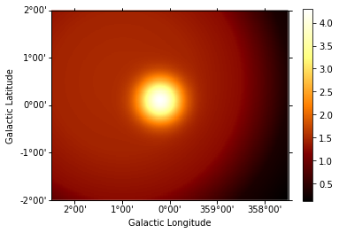
npred = evaluator.compute_npred()
npred_map = WcsNDMap(geom, npred)
In [14]:
npred_map.sum_over_axes().plot(add_cbar=True);
In [15]:
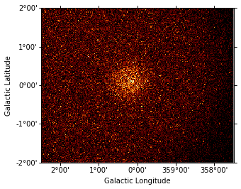
# This one line is the core of how to simulate data when
# using binned simulation / analysis: you Poisson fluctuate
# npred to obtain simulated observed counts.
# Compute counts as a Poisson fluctuation
rng = np.random.RandomState(seed=42)
counts = rng.poisson(npred)
counts_map = WcsNDMap(geom, counts)
In [16]:
counts_map.sum_over_axes().plot();
Fit
Now let’s analyse the simulated data. Here we just fit it again with the same model we had before, but you could do any analysis you like here, e.g. fit a different model, or do a region-based analysis, …
In [17]:
# Define sky model to fit the data
spatial_model = SkyGaussian(lon_0="0 deg", lat_0="0 deg", sigma="1 deg")
spectral_model = PowerLaw(
    index=2, amplitude="1e-11 cm-2 s-1 TeV-1", reference="1 TeV"
)
model = SkyModel(spatial_model=spatial_model, spectral_model=spectral_model)
print(model)
SkyModel

spatial_model = SkyGaussian

Parameters:

         name   value   error unit min max
        ----- --------- ----- ---- --- ---
        lon_0 0.000e+00   nan  deg nan nan
        lat_0 0.000e+00   nan  deg nan nan
        sigma 1.000e+00   nan  deg nan nan

spectral_model = PowerLaw

Parameters:

           name     value   error       unit         min    max
        --------- --------- ----- --------------- --------- ---
            index 2.000e+00   nan                       nan nan
        amplitude 1.000e-11   nan 1 / (cm2 s TeV)       nan nan
        reference 1.000e+00   nan             TeV 0.000e+00 nan
In [18]:
%%time
fit = MapFit(
    model=model,
    counts=counts_map,
    exposure=exposure,
    background=background,
    psf=psf_kernel,
)

result = fit.run(optimize_opts={"print_level": 1})
| FCN = 268093.5231869054 | TOTAL NCALL = 313 | NCALLS = 313 |
| EDM = 1.2783287759261633e-05 | GOAL EDM = 1e-05 | UP = 1.0 |
| Valid | Valid Param | Accurate Covar | PosDef | Made PosDef |
| True | True | True | True | False |
| Hesse Fail | HasCov | Above EDM | Reach calllim | |
| False | True | False | False |
| + | Name | Value | Hesse Error | Minos Error- | Minos Error+ | Limit- | Limit+ | Fixed? |
| 0 | par_000_lon_0 | 0.209775 | 0.00854235 | No | ||||
| 1 | par_001_lat_0 | 0.0952569 | 0.00859662 | No | ||||
| 2 | par_002_sigma | -0.290008 | 0.00592014 | No | ||||
| 3 | par_003_index | 2.9923 | 0.0291751 | No | ||||
| 4 | par_004_amplitude | 1.01247 | 0.0494739 | No | ||||
| 5 | par_005_reference | 1 | 1 | 0 | Yes |
CPU times: user 16.9 s, sys: 858 ms, total: 17.7 s
Wall time: 17.8 s
True model:
In [19]:
print(sky_model)
SkyModel

spatial_model = SkyGaussian

Parameters:

         name   value   error unit min max
        ----- --------- ----- ---- --- ---
        lon_0 2.000e-01   nan  deg nan nan
        lat_0 1.000e-01   nan  deg nan nan
        sigma 3.000e-01   nan  deg nan nan

spectral_model = PowerLaw

Parameters:

           name     value   error       unit         min    max
        --------- --------- ----- --------------- --------- ---
            index 3.000e+00   nan                       nan nan
        amplitude 1.000e-11   nan 1 / (cm2 s TeV)       nan nan
        reference 1.000e+00   nan             TeV 0.000e+00 nan
Best-fit model:
In [20]:
print(result.model)
SkyModel

spatial_model = SkyGaussian

Parameters:

         name   value      error   unit min max
        ----- ---------- --------- ---- --- ---
        lon_0  2.098e-01 8.542e-03  deg nan nan
        lat_0  9.526e-02 8.597e-03  deg nan nan
        sigma -2.900e-01 5.920e-03  deg nan nan

Covariance:

         name   lon_0      lat_0      sigma
        ----- ---------- ---------- ----------
        lon_0  7.297e-05 -1.472e-07 -1.032e-06
        lat_0 -1.472e-07  7.390e-05 -6.568e-07
        sigma -1.032e-06 -6.568e-07  3.505e-05

spectral_model = PowerLaw

Parameters:

           name     value     error         unit         min    max
        --------- --------- --------- --------------- --------- ---
            index 2.992e+00 2.918e-02                       nan nan
        amplitude 1.012e-11 4.947e-13 1 / (cm2 s TeV)       nan nan
        reference 1.000e+00 0.000e+00             TeV 0.000e+00 nan

Covariance:

           name     index    amplitude  reference
        --------- ---------- ---------- ---------
            index  8.512e-04 -1.205e-14 0.000e+00
        amplitude -1.205e-14  2.448e-25 0.000e+00
        reference  0.000e+00  0.000e+00 0.000e+00
In [21]:
# TODO: show e.g. how to make a residual image
iminuit
What we have done for now is to write a very thin wrapper for http://iminuit.readthedocs.io/ as a fitting backend. This is just a prototype, we will improve this interface and add other fitting backends (e.g. Sherpa or scipy.optimize or emcee or …)
As a power-user, you can access fit._iminuit and get the full power
of what is developed there already. E.g. the fit.fit() call ran
Minuit.migrad() and Minuit.hesse() in the background, and you
have access to e.g. the covariance matrix, or can check a likelihood
profile, or can run Minuit.minos() to compute asymmetric errors or …
In [22]:
# Check correlation between model parameters
# As expected in this simple case,
# spatial parameters are uncorrelated,
# but the spectral model amplitude and index are correlated as always
fit.minuit.print_matrix()
| + | par_000_lon_0 | par_001_lat_0 | par_002_sigma | par_003_index | par_004_amplitude |
| par_000_lon_0 | 1.00 | -0.00 | -0.02 | -0.01 | 0.01 |
| par_001_lat_0 | -0.00 | 1.00 | -0.01 | 0.01 | -0.01 |
| par_002_sigma | -0.02 | -0.01 | 1.00 | 0.02 | -0.31 |
| par_003_index | -0.01 | 0.01 | 0.02 | 1.00 | -0.83 |
| par_004_amplitude | 0.01 | -0.01 | -0.31 | -0.83 | 1.00 |
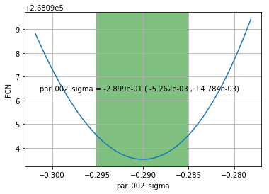
In [23]:
# You can use likelihood profiles to check if your model is
# well constrained or not, and if the fit really converged
fit.minuit.draw_profile("par_002_sigma");