NaimaSpectralModel¶

class gammapy.modeling.models.NaimaSpectralModel(radiative_model, distance=<Quantity 1. kpc>, seed=None)[source]¶

Bases: gammapy.modeling.models.SpectralModel

A wrapper for Naima models.

This class provides an interface with the models defined in the models module. The model accepts as a positional argument a Naima radiative model instance, used to compute the non-thermal emission from populations of relativistic electrons or protons due to interactions with the ISM or with radiation and magnetic fields.

One of the advantages provided by this class consists in the possibility of performing a maximum likelihood spectral fit of the model’s parameters directly on observations, as opposed to the MCMC fit to flux points featured in Naima. All the parameters defining the parent population of charged particles are stored as Parameter and left free by default. In case that the radiative model is ` ~naima.radiative.Synchrotron`, the magnetic field strength may also be fitted. Parameters can be freezed/unfreezed before the fit, and maximum/minimum values can be set to limit the parameters space to the physically interesting region.

Parameters:

radiative_model : BaseRadiative: An instance of a radiative model defined in models
distance : Quantity, optional: Distance to the source. If set to 0, the intrinsic differential luminosity will be returned. Default is 1 kpc
seed : str or list of str, optional: Seed photon field(s) to be considered for the radiative_model flux computation, in case of a InverseCompton model. It can be a subset of the seed_photon_fields list defining the radiative_model. Default is the whole list of photon fields

Examples

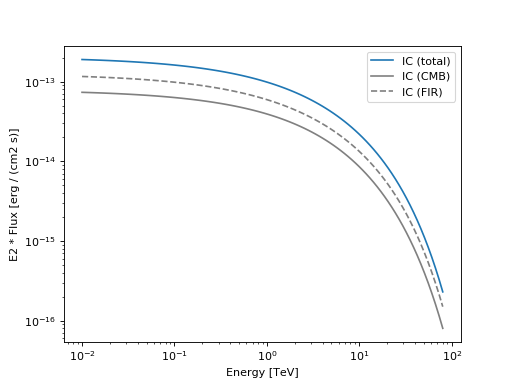
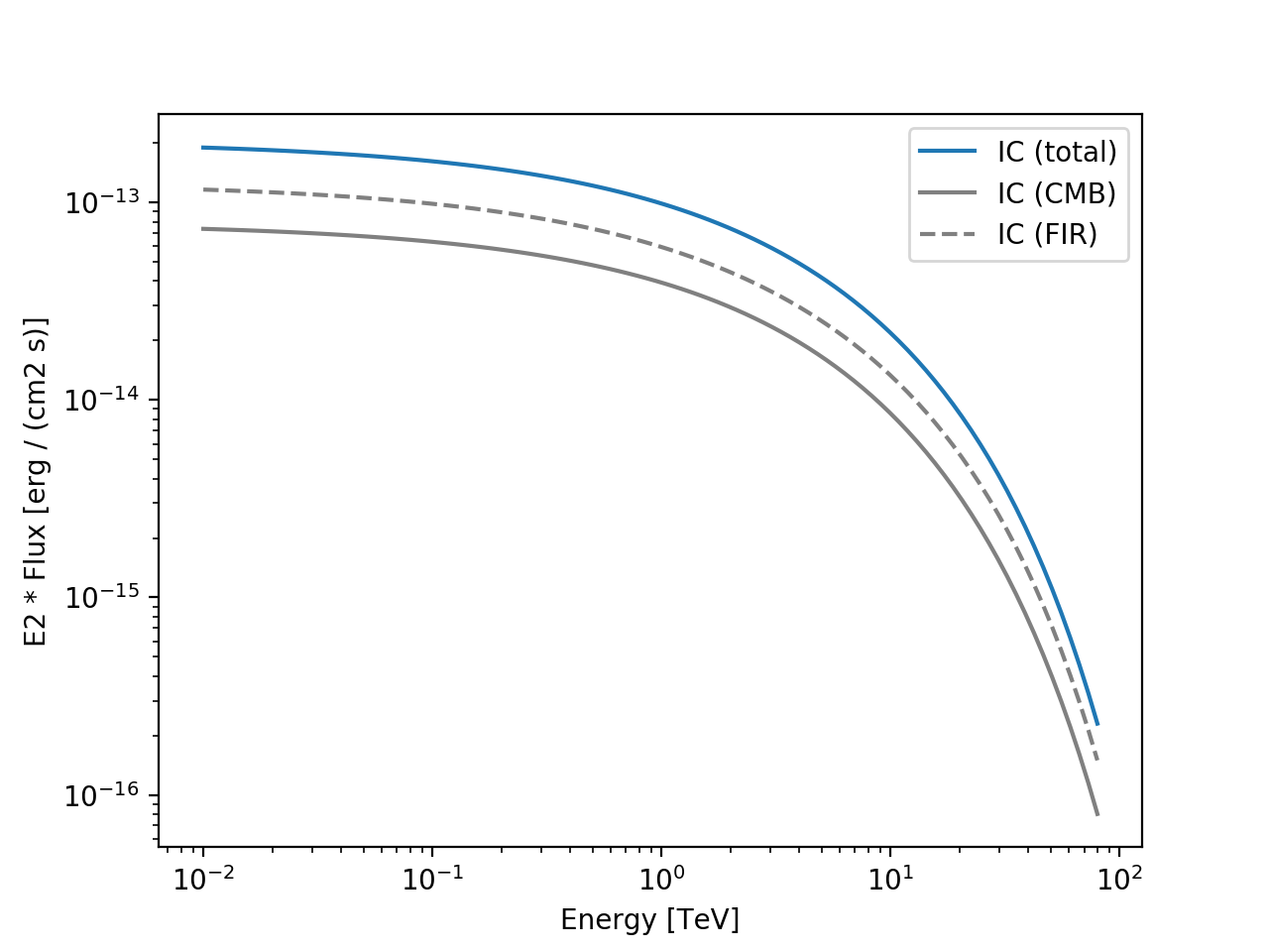
Create and plot a spectral model that convolves an ExpCutoffPowerLawSpectralModel electron distribution with an InverseCompton radiative model, in the presence of multiple seed photon fields.

import naima
from gammapy.modeling.models import NaimaSpectralModel
import astropy.units as u
import matplotlib.pyplot as plt

particle_distribution = naima.models.ExponentialCutoffPowerLaw(1e30 / u.eV, 10 * u.TeV, 3.0, 30 * u.TeV)
radiative_model = naima.radiative.InverseCompton(
    particle_distribution,
    seed_photon_fields=[
        "CMB",
        ["FIR", 26.5 * u.K, 0.415 * u.eV / u.cm ** 3],
    ],
    Eemin=100 * u.GeV,
)

model = NaimaSpectralModel(radiative_model, distance=1.5 * u.kpc)

opts = {
    "energy_range" : [10 * u.GeV, 80 * u.TeV],
    "energy_power" : 2,
    "flux_unit" : "erg-1 cm-2 s-1",
}

# Plot the total inverse Compton emission
model.plot(label='IC (total)', **opts)

# Plot the separate contributions from each seed photon field
for seed, ls in zip(['CMB','FIR'], ['-','--']):
    model = NaimaSpectralModel(radiative_model, seed=seed, distance=1.5 * u.kpc)
    model.plot(label="IC ({})".format(seed), ls=ls, color="gray", **opts)

plt.legend(loc='best')
plt.show()

(png, hires.png, pdf)

../_images/gammapy-modeling-models-NaimaSpectralModel-1.png

Attributes Summary

`parameters`	Parameters (`Parameters`)
`tag`

Methods Summary

`__call__`(self, energy)	Call self as a function.
`copy`(self)	A deep copy.
`create`(tag, \args, \\*kwargs)	Create a model instance.
`energy_flux`(self, emin, emax, \\kwargs)	Compute energy flux in given energy range.
`energy_flux_error`(self, emin, emax, \\kwargs)	Compute energy flux in given energy range with error propagation.
`evaluate`(self, energy, \\kwargs)	Evaluate the model.
`evaluate_error`(self, energy)	Evaluate spectral model with error propagation.
`from_dict`(data)
`integral`(self, emin, emax, \\kwargs)	Integrate spectral model numerically.
`integral_error`(self, emin, emax, \\kwargs)	Integrate spectral model numerically with error propagation.
`inverse`(self, value[, emin, emax])	Return energy for a given function value of the spectral model.
`plot`(self, energy_range[, ax, energy_unit, …])	Plot spectral model curve.
`plot_error`(self, energy_range[, ax, …])	Plot spectral model error band.
`spectral_index`(self, energy[, epsilon])	Compute spectral index at given energy.
`to_dict`(self)

Attributes Documentation

parameters¶: Parameters (Parameters)

tag = 'NaimaSpectralModel'¶

Methods Documentation

__call__(self, energy)¶: Call self as a function.

copy(self)¶: A deep copy.

static create(tag, *args, **kwargs)¶

Create a model instance.

Examples

>>> from gammapy.modeling import Model
>>> spectral_model = Model.create("PowerLaw2SpectralModel", amplitude="1e-10 cm-2 s-1", index=3)
>>> type(spectral_model)
gammapy.modeling.models.spectral.PowerLaw2SpectralModel

energy_flux(self, emin, emax, **kwargs)¶

Compute energy flux in given energy range.

\[G(E_{min}, E_{max}) = \int_{E_{min}}^{E_{max}} E \phi(E) dE\]

Parameters:	emin, emax : `Quantity` Lower and upper bound of integration range. **kwargs : dict Keyword arguments passed to func:`integrate_spectrum`

energy_flux_error(self, emin, emax, **kwargs)¶

Compute energy flux in given energy range with error propagation.

\[G(E_{min}, E_{max}) = \int_{E_{min}}^{E_{max}} E \phi(E) dE\]

Parameters:	emin, emax : `Quantity` Lower bound of integration range. **kwargs : dict Keyword arguments passed to `integrate_spectrum()`
Returns:	energy_flux, energy_flux_error : tuple of `Quantity` Tuple of energy flux and energy flux error.

evaluate(self, energy, **kwargs)[source]¶: Evaluate the model.

evaluate_error(self, energy)[source]¶

Evaluate spectral model with error propagation.

Parameters:	energy : `Quantity` Energy at which to evaluate
Returns:	flux, flux_error : tuple of `Quantity` Tuple of flux and flux error.

classmethod from_dict(data)¶

integral(self, emin, emax, **kwargs)¶

Integrate spectral model numerically.

\[F(E_{min}, E_{max}) = \int_{E_{min}}^{E_{max}} \phi(E) dE\]

If array input for emin and emax is given you have to set intervals=True if you want the integral in each energy bin.

Parameters:	emin, emax : `Quantity` Lower and upper bound of integration range. **kwargs : dict Keyword arguments passed to `integrate_spectrum()`

integral_error(self, emin, emax, **kwargs)¶

Integrate spectral model numerically with error propagation.

Parameters:	emin, emax : `Quantity` Lower adn upper bound of integration range. **kwargs : dict Keyword arguments passed to func:`integrate_spectrum`
Returns:	integral, integral_error : tuple of `Quantity` Tuple of integral flux and integral flux error.

inverse(self, value, emin=<Quantity 0.1 TeV>, emax=<Quantity 100. TeV>)¶

Return energy for a given function value of the spectral model.

Calls the scipy.optimize.brentq numerical root finding method.

Parameters:	value : `Quantity` Function value of the spectral model. emin : `Quantity` Lower bracket value in case solution is not unique. emax : `Quantity` Upper bracket value in case solution is not unique.
Returns:	energy : `Quantity` Energies at which the model has the given `value`.

plot(self, energy_range, ax=None, energy_unit='TeV', flux_unit='cm-2 s-1 TeV-1', energy_power=0, n_points=100, **kwargs)¶

Plot spectral model curve.

kwargs are forwarded to matplotlib.pyplot.plot

By default a log-log scaling of the axes is used, if you want to change the y axis scaling to linear you can use:

from gammapy.modeling.models import ExpCutoffPowerLawSpectralModel
from astropy import units as u

pwl = ExpCutoffPowerLawSpectralModel()
ax = pwl.plot(energy_range=(0.1, 100) * u.TeV)
ax.set_yscale('linear')

Parameters:	ax : `Axes`, optional Axis energy_range : `Quantity` Plot range energy_unit : str, `Unit`, optional Unit of the energy axis flux_unit : str, `Unit`, optional Unit of the flux axis energy_power : int, optional Power of energy to multiply flux axis with n_points : int, optional Number of evaluation nodes
Returns:	ax : `Axes`, optional Axis

plot_error(self, energy_range, ax=None, energy_unit='TeV', flux_unit='cm-2 s-1 TeV-1', energy_power=0, n_points=100, **kwargs)¶

Plot spectral model error band.

Note

This method calls ax.set_yscale("log", nonposy='clip') and ax.set_xscale("log", nonposx='clip') to create a log-log representation. The additional argument nonposx='clip' avoids artefacts in the plot, when the error band extends to negative values (see also https://github.com/matplotlib/matplotlib/issues/8623).

When you call plt.loglog() or plt.semilogy() explicitely in your plotting code and the error band extends to negative values, it is not shown correctly. To circumvent this issue also use plt.loglog(nonposx='clip', nonposy='clip') or plt.semilogy(nonposy='clip').

Parameters:

ax : Axes, optional: Axis
energy_range : Quantity: Plot range
energy_unit : str, Unit, optional: Unit of the energy axis
flux_unit : str, Unit, optional: Unit of the flux axis
energy_power : int, optional: Power of energy to multiply flux axis with
n_points : int, optional: Number of evaluation nodes
**kwargs : dict: Keyword arguments forwarded to matplotlib.pyplot.fill_between

Returns:

ax : Axes, optional: Axis

spectral_index(self, energy, epsilon=1e-05)¶

Compute spectral index at given energy.

Parameters:	energy : `Quantity` Energy at which to estimate the index epsilon : float Fractional energy increment to use for determining the spectral index.
Returns:	index : float Estimated spectral index.

to_dict(self)¶