Computation of the CTA sensitivity¶

Introduction¶

This notebook explains how to derive the CTA sensitivity for a point-like IRF at a fixed zenith angle and fixed offset. The significativity is computed for the 1D analysis (On-OFF regions) and the LiMa formula.

We will be using the following Gammapy classes:

Setup¶

As usual, we’ll start with some setup …

In [1]:

%matplotlib inline
import matplotlib.pyplot as plt

In [2]:

from gammapy.irf import CTAPerf
from gammapy.spectrum import SensitivityEstimator

Load IRFs¶

First load the CTA IRFs.

In [3]:

filename = "$GAMMAPY_EXTRA/datasets/cta/perf_prod2/point_like_non_smoothed/South_5h.fits.gz"
irf = CTAPerf.read(filename)

Compute sensitivity¶

Choose a few parameters, then run the sentitivity computation.

In [4]:

sensitivity_estimator = SensitivityEstimator(irf=irf, livetime="5h")
sensitivity_estimator.run()

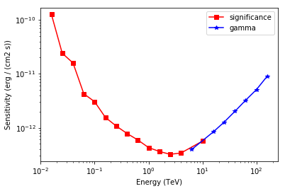
Results¶

The results are given as an Astropy table.

In [5]:

# Show the results table
sensitivity_estimator.results_table

Out[5]:

Table length=21

energy	e2dnde	excess	background	criterion
TeV	erg / (cm2 s)
float32	float64	float64	float32	str12
0.0158489	1.26569e-10	339.143	3703.48	significance
0.0251189	2.41235e-11	311.106	3106.66	significance
0.0398107	1.5914e-11	459.213	6852.06	significance
0.0630957	4.26714e-12	163.204	825.794	significance
0.1	3.04454e-12	169.361	891.645	significance
0.158489	1.55368e-12	90.0926	236.905	significance
0.251189	1.0771e-12	51.5349	69.8381	significance
0.398107	7.83236e-13	35.6905	29.8996	significance
0.630957	5.93807e-13	26.4005	14.2506	significance
1	4.28759e-13	18.1072	5.11857	significance
1.58489	3.62852e-13	15.6871	3.31032	significance
2.51189	3.21257e-13	11.7016	1.17059	significance
3.98107	3.39152e-13	12.0962	1.33607	significance
6.30957	3.9511e-13	10	0.424068	gamma
10	5.65043e-13	10.898	0.865076	significance
15.8489	8.36566e-13	10	0.216136	gamma
25.1189	1.26771e-12	10	0.00979249	gamma
39.8107	2.00893e-12	10	0.0053102	gamma
63.0957	3.24246e-12	10	0.00170479	gamma
100	5.10213e-12	10	0.00101395	gamma
158.489	9.04831e-12	10	0.00566093	gamma

In [6]:

# Save it to file (could use e.g. format of CSV or ECSV or FITS)
# sensitivity_estimator.results_table.write('sensitivity.ecsv', format='ascii.ecsv')

In [7]:

# Plot the sensitivity curve
t = sensitivity_estimator.results_table

is_s = t["criterion"] == "significance"
plt.plot(
    t["energy"][is_s],
    t["e2dnde"][is_s],
    "s-",
    color="red",
    label="significance",
)

is_g = t["criterion"] == "gamma"
plt.plot(
    t["energy"][is_g], t["e2dnde"][is_g], "*-", color="blue", label="gamma"
)

plt.loglog()
plt.xlabel("Energy ({})".format(t["energy"].unit))
plt.ylabel("Sensitivity ({})".format(t["e2dnde"].unit))
plt.legend();

../_images/notebooks_cta_sensitivity_13_0.png

Exercises¶

Also compute the sensitivity for a 20 hour observation
Compare how the sensitivity differs between 5 and 20 hours by plotting the ratio as a function of energy.