Spectrum simulation for CTA¶

A quick example how to simulate and fit a spectrum for the Cherenkov Telescope Array (CTA).

We will use the following classes:

Setup¶

In [1]:

%matplotlib inline
import matplotlib.pyplot as plt

In [2]:

import numpy as np
import astropy.units as u
from gammapy.irf import EnergyDispersion, EffectiveAreaTable
from gammapy.spectrum import SpectrumSimulation, SpectrumFit
from gammapy.spectrum.models import PowerLaw
from gammapy.irf import CTAIrf

Simulation¶

In [3]:

# Define simulation parameters parameters
livetime = 1 * u.h
offset = 0.5 * u.deg
# Energy from 0.1 to 100 TeV with 10 bins/decade
energy = np.logspace(-1, 2, 31) * u.TeV

In [4]:

# Define spectral model
model = PowerLaw(
    index=2.1,
    amplitude=2.5e-12 * u.Unit("cm-2 s-1 TeV-1"),
    reference=1 * u.TeV,
)

In [5]:

# Load IRFs
filename = (
    "$GAMMAPY_DATA/cta-1dc/caldb/data/cta/1dc/bcf/South_z20_50h/irf_file.fits"
)
cta_irf = CTAIrf.read(filename)

In [6]:

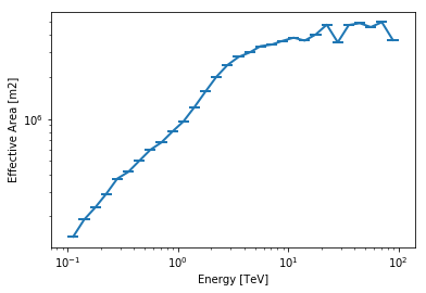
aeff = cta_irf.aeff.to_effective_area_table(offset=offset, energy=energy)
aeff.plot()
plt.loglog()
print(cta_irf.aeff.data)

NDDataArray summary info
energy         : size =    42, min =  0.014 TeV, max = 177.828 TeV
offset         : size =     6, min =  0.500 deg, max =  5.500 deg
Data           : size =   252, min =  0.000 m2, max = 5371581.000 m2

../_images/notebooks_spectrum_simulation_cta_9_1.png

In [7]:

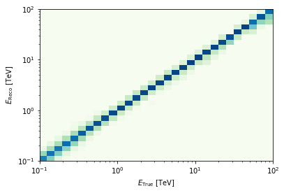
edisp = cta_irf.edisp.to_energy_dispersion(
    offset=offset, e_true=energy, e_reco=energy
)
edisp.plot_matrix()
print(edisp.data)

NDDataArray summary info
e_true         : size =    30, min =  0.112 TeV, max = 89.125 TeV
e_reco         : size =    30, min =  0.112 TeV, max = 89.125 TeV
Data           : size =   900, min =  0.000, max =  0.926

../_images/notebooks_spectrum_simulation_cta_10_1.png

In [8]:

# Simulate data
sim = SpectrumSimulation(
    aeff=aeff, edisp=edisp, source_model=model, livetime=livetime
)
sim.simulate_obs(seed=42, obs_id=0)

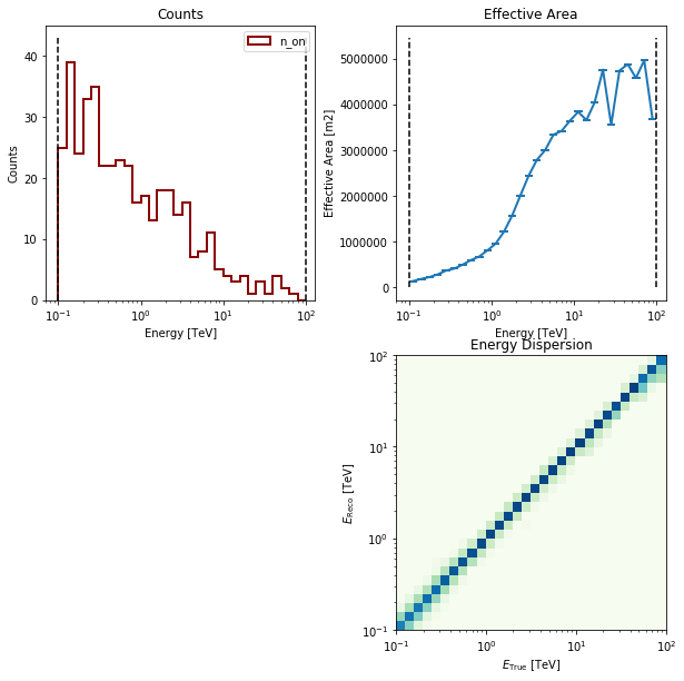
In [9]:

sim.obs.peek()
print(sim.obs)

*** Observation summary report ***
Observation Id: 0
Livetime: 1.000 h
On events: 411
Off events: 0
Alpha: 1.000
Bkg events in On region: 0.00
Excess: 411.00
Excess / Background: inf
Gamma rate: 411.00 1 / h
Bkg rate: 0.00 1 / min
Sigma: nan
energy range: 0.10 TeV - 100.00 TeV

../_images/notebooks_spectrum_simulation_cta_12_1.png

Spectral analysis¶

Now that we have some simulated CTA counts spectrum, let’s analyse it.

In [10]:

# Fit data
fit = SpectrumFit(obs_list=sim.obs, model=model, stat="cash")
fit.run()
result = fit.result[0]

In [11]:

print(result)


Fit result info
---------------
Model: PowerLaw

Parameters:

           name     value     error         unit         min    max
        --------- --------- --------- --------------- --------- ---
            index 2.116e+00 3.446e-02                       nan nan
        amplitude 2.382e-12 1.205e-13 1 / (cm2 s TeV)       nan nan
        reference 1.000e+00 0.000e+00             TeV 0.000e+00 nan

Covariance:

           name     index    amplitude  reference
        --------- ---------- ---------- ---------
            index  1.188e-03 -9.160e-16 0.000e+00
        amplitude -9.160e-16  1.451e-26 0.000e+00
        reference  0.000e+00  0.000e+00 0.000e+00

Statistic: -1591.397 (cash)
Fit Range: [   0.1  100. ] TeV

In [12]:

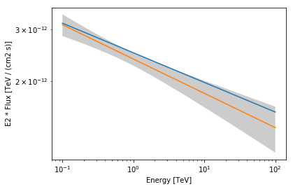
energy_range = [0.1, 100] * u.TeV
model.plot(energy_range=energy_range, energy_power=2)
result.model.plot(energy_range=energy_range, energy_power=2)
result.model.plot_error(energy_range=energy_range, energy_power=2);

../_images/notebooks_spectrum_simulation_cta_16_0.png

Exercises¶

Change the observation time to something longer or shorter. Does the observation and spectrum results change as you expected?
Change the spectral model, e.g. add a cutoff at 5 TeV, or put a steep-spectrum source with spectral index of 4.0

In [13]:

# Start the exercises here!

What next?¶

In this tutorial we simulated and analysed the spectrum of source using CTA prod 2 IRFs.

If you’d like to go further, please see the other tutorial notebooks.