Instrument Response Functions (DL3)#

Typically the IRFs are stored in the form of multidimensional tables giving the response functions such as the distribution of gamma-like events or the probability density functions of the reconstructed energy and position.

Expected number of detected events#

To model the expected number of events a gamma-ray source should produce on a detector, one has to model its effect using an instrument response function (IRF). In general, such a function gives:

for the residual instrumental background events, the probability to detect an event at reconstructed position \(p\) and energy \(E\),
for the expected event number from a gamma-ray source, the probability to detect a photon emitted from true position \(p_{\rm true}\) on the sky and true energy \(E_{\rm true}\) at reconstructed position \(p\) and energy \(E\) and the effective collection area of the detector at position \(p_{\rm true}\) on the sky and true energy \(E_{\rm true}\).

We can write the expected number of detected events in a bin [\({\rm d}p,\,{\rm d}E\)]:

\[N(p, E) \, {\rm d}p {\rm d}E = {N(p, E)_{\rm bkg}} \, {\rm d}p {\rm d}E + {N(p, E)_{\rm src}} \, {\rm d}p {\rm d}E\]

with:

\[{N(p, E)_{\rm bkg}}\, {\rm d}p {\rm d}E = t_{\rm obs} \int_{E} {\rm d}E \, \int_{p} {\rm d}p \, {\rm Bkg}(p, E)\]

where \({\rm Bkg}(p, E)\) is the instrument response on the residual instrumental background rate (unit: \({\rm s}^{-1}\,{\rm sr}^{-1}\))

and with:

\[{N(p, E)_{\rm src}} \, {\rm d}p {\rm d}E = t_{\rm obs} \int_{E_{\rm true}} {\rm d}E_{\rm true} \, \int_{p_{\rm true}} {\rm d}p_{\rm true} \, R(p, E|p_{\rm true}, E_{\rm true}) \times \Phi(p_{\rm true}, E_{\rm true})\]

where:

\(R(p, E| p_{\rm true}, E_{\rm true})\) is the instrument response (unit: \({\rm m}^2\,{\rm TeV}^{-1}\))
\(\Phi(p_{\rm true}, E_{\rm true})\) is the sky flux model (unit: \({\rm m}^{-2}\,{\rm s}^{-1}\,{\rm TeV}^{-1}\,{\rm sr}^{-1}\))
\(t_{\rm obs}\) is the observation time: (unit: \({\rm s}\))

Residual instrumental background rate#

The response \({\rm Bkg}(p, E)\) is coming from atmospheric cosmic-rays that are mis-classified as gamma-ray candidates. They originate from hadrons (mainly protons) and leptons (mainly electrons), depending on the energy. These events constitute an irreducible source of background when studying gamma-ray emissions; they are also subjects of analysis (e.g. cosmic ray spectrum, charge composition, isotropy and dipole search), which is beyond the scope of this documentation.

\({\rm Bkg}(p, E)\) predicts the rate of such events. This response is complex to derive by the observatories, in order to cover the whole observational phase space (p, E) and the instrument variations (atmosphere and detectors). Most of the time, real events are used to build such instrument response. This rate is then delivered by the observatories. In the DL3 format, this IRF is distributed for each observing run for the IACT observatories.

For a standard 3D Analysis as implemented in Gammapy (with a FoVBackgroundModel) or to make maps with the RingBackgroundMaker (see Ring background), this IRF is necessary. If this is missing, one can use a measurement of the OFF counts in the FoV, e.g. as used in 1D Analysis (e.g. Reflected regions background).

Note that this function is expressed as function of the reconstructed quantities (here \(p\) and \(E\)).

Factorisation of the gamma-ray IRFs#

Most of the time, in high level gamma-ray data (DL3), we assume that the gamma-ray instrument response can be simplified as the product of three independent functions:

\[R(p, E|p_{\rm true}, E_{\rm true}) = A_{\rm eff}(p_{\rm true}, E_{\rm true}) \times PSF(p|p_{\rm true}, E_{\rm true}) \times E_{\rm disp}(E|p_{\rm true}, E_{\rm true}),\]

where:

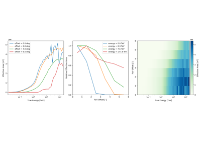
\(A_{\rm eff}(p_{\rm true}, E_{\rm true})\) is the effective collection area of the detector (unit: \({\rm m}^2\)). It is the product of the detector collection area times its detection efficiency at true energy \(E_{\rm true}\) and position \(p_{\rm true}\).
\(PSF(p|p_{\rm true}, E_{\rm true})\) is the point spread function (unit: \({\rm sr}^{-1}\)). It gives the probability of measuring a direction \(p\) when the true direction is \(p_{\rm true}\) and the true energy is \(E_{\rm true}\). Gamma-ray instruments consider the probability density of the angular separation between true and reconstructed directions \(\delta p = p_{\rm true} - p\), i.e. \(PSF(\delta p|p_{\rm true}, E_{\rm true})\).
\(E_{\rm disp}(E|p_{\rm true}, E_{\rm true})\) is the energy dispersion (unit: \({\rm TeV}^{-1}\)). It gives the probability to reconstruct the photon at energy \(E\) when the true energy is \(E_{\rm true}\) and the true position \(p_{\rm true}\). Gamma-ray instruments consider the probability density of the migration \(\mu=\frac{E}{E_{\rm true}}\), i.e. \(E_{\rm disp}(\mu|p_{\rm true}, E_{\rm true})\).

The implicit assumption here is that energy dispersion and PSF are completely independent. This is not totally valid in some situations.

Note that all these functions are expressed as function of the true quantities (here \(p_{\rm true}\) and \(E_{\rm true}\)).

These functions are obtained through Monte-Carlo simulations of gamma-ray showers for different observing conditions, e.g. detector configuration, zenith angle of the pointing position, detector state and different event reconstruction and selection schemes. In the DL3 format, the IRF are distributed for each observing run.

Need of four individual responses#

In order to statistically estimate a gamma-ray source model, the expected number of detected events in each [\({\rm d}p,\,{\rm d}E\)] bin are tested in regards to the measured events (see Fit statistics). To make such statistical studies, the four individual responses are then mandatory to be delivered with a data release by the observatories.

Further details on individuals responses and how they are implemented in Gammapy are given in:

Most of the formats defined at IRFs are supported. Currently, there is some support for Fermi-LAT and other instruments, with ongoing efforts to improve this.

Most users will not use gammapy.irf directly, but will instead use IRFs as part of their spectrum, image or cube analysis (via e.g. the MapDatasetMaker during the data reduction, see Data reduction (DL3 to DL4)).

IRF axis naming#

In the IRF classes, we use the following axis naming convention:

Variable	Definition
`energy`	Reconstructed energy axis (\(E\))
`energy_true`	True energy axis (\(E_{\rm true}\))
`offset`	Field of view offset from center (\(p_{\rm true}\))
`fov_lon`	Field of view longitude
`fov_lat`	Field of view latitude
`migra`	Energy migration (\(\mu\))
`rad`	Offset angle from source position (\(\delta p\))