Note
Go to the end to download the full example code or to run this example in your browser via Binder.
Point source sensitivity#
Estimate the CTAO sensitivity for a point-like IRF at a fixed zenith angle and fixed offset.
Introduction#
This notebook explains how to estimate the CTAO sensitivity for a point-like IRF at a fixed zenith angle and fixed offset, using the full containment IRFs distributed for the CTA 1DC. The significance is computed for a 1D analysis (ON-OFF regions) with the Li & Ma formula.
We use here an approximate approach with an energy dependent integration radius to take into account the variation of the PSF. We will first determine the 1D IRFs including a containment correction.
We will be using the following Gammapy class:
from cycler import cycler
import numpy as np
import astropy.units as u
from astropy.coordinates import SkyCoord

# %matplotlib inline
from regions import CircleSkyRegion
import matplotlib.pyplot as plt
Setup#
As usual, we’ll start with some setup …
from IPython.display import display
from gammapy.data import FixedPointingInfo, Observation, observatory_locations
from gammapy.datasets import SpectrumDataset, SpectrumDatasetOnOff
from gammapy.estimators import FluxPoints, SensitivityEstimator
from gammapy.irf import load_irf_dict_from_file
from gammapy.makers import SpectrumDatasetMaker
from gammapy.maps import MapAxis, RegionGeom
from gammapy.maps.axes import UNIT_STRING_FORMAT
Define analysis region and energy binning#
Here we assume a source at 0.5 degree from pointing position. We perform a simple energy independent extraction for now with a radius of 0.1 degree.
energy_axis = MapAxis.from_energy_bounds(0.03 * u.TeV, 30 * u.TeV, nbin=20)
energy_axis_true = MapAxis.from_energy_bounds(
    0.01 * u.TeV, 100 * u.TeV, nbin=100, name="energy_true"
)

pointing = SkyCoord(ra=0 * u.deg, dec=0 * u.deg)
pointing_info = FixedPointingInfo(fixed_icrs=pointing)
offset = 0.5 * u.deg

source_position = pointing.directional_offset_by(0 * u.deg, offset)
on_region_radius = 0.1 * u.deg
on_region = CircleSkyRegion(source_position, radius=on_region_radius)

geom = RegionGeom.create(on_region, axes=[energy_axis])
empty_dataset = SpectrumDataset.create(geom=geom, energy_axis_true=energy_axis_true)
Load IRFs and prepare dataset#
We extract the 1D IRFs from the full 3D IRFs provided by CTAO.
irfs = load_irf_dict_from_file(
    "$GAMMAPY_DATA/cta-1dc/caldb/data/cta/1dc/bcf/South_z20_50h/irf_file.fits"
)
location = observatory_locations["ctao_south"]
livetime = 50.0 * u.h
obs = Observation.create(
    pointing=pointing_info, irfs=irfs, livetime=livetime, location=location
)
/home/runner/work/gammapy-docs/gammapy-docs/gammapy/.tox/build_docs/lib/python3.12/site-packages/astropy/units/core.py:2102: UnitsWarning: '1/s/MeV/sr' did not parse as fits unit: Numeric factor not supported by FITS If this is meant to be a custom unit, define it with 'u.def_unit'. To have it recognized inside a file reader or other code, enable it with 'u.add_enabled_units'. For details, see https://docs.astropy.org/en/latest/units/combining_and_defining.html
  warnings.warn(msg, UnitsWarning)
Initiate and run the SpectrumDatasetMaker.
Note that here we ensure containment_correction=False which allows us to
apply our own containment correction in the next part of the tutorial.
spectrum_maker = SpectrumDatasetMaker(
    selection=["exposure", "edisp", "background"],
    containment_correction=False,
)
dataset = spectrum_maker.run(empty_dataset, obs)
Now we correct for the energy dependent region size.
Note: In the calculation of the containment radius, we use the point spread function which is defined dependent on true energy to compute the correction we apply in reconstructed energy, thus neglecting the energy dispersion in this step.
Start by correcting the exposure:
containment = 0.68
dataset.exposure *= containment
Next, correct the background estimation.
Warning
This neglects the energy dispersion by computing the containment radius from the PSF in true energy but using the reco energy axis.
on_radii = obs.psf.containment_radius(
    energy_true=energy_axis.center, offset=offset, fraction=containment
)
factor = (1 - np.cos(on_radii)) / (1 - np.cos(on_region_radius))
dataset.background *= factor.value.reshape((-1, 1, 1))
Finally, define a SpectrumDatasetOnOff with an alpha of 0.2.
The off counts are created from the background model:
dataset_on_off = SpectrumDatasetOnOff.from_spectrum_dataset(
    dataset=dataset, acceptance=1, acceptance_off=5
)
Compute sensitivity#
We impose a minimal number of expected signal counts of 10 per bin and a minimal significance of 5 per bin. The excess must also be larger than 5% of the background.
We assume an alpha of 0.2 (ratio between ON and OFF area). We then run the sensitivity estimator.
These are the conditions imposed in standard CTAO sensitivity computations.
sensitivity_estimator = SensitivityEstimator(
    gamma_min=10,
    n_sigma=5,
    bkg_syst_fraction=0.05,
)
sensitivity_table = sensitivity_estimator.run(dataset_on_off)
Results#
The results are given as a Table, which can be written to
disk utilising the usual write method.
A column criterion allows us
to distinguish bins where the significance is limited by the signal
statistical significance from bins where the sensitivity is limited by
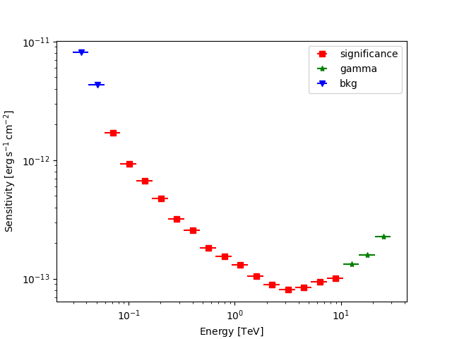
the number of signal counts. This is visible in the plot below.
display(sensitivity_table)
  e_ref     e_min     e_max       e2dnde     excess background  criterion
   TeV       TeV       TeV    erg / (s cm2)
--------- --------- --------- ------------- ------- ---------- ------------
0.0356551      0.03 0.0423761    8.0756e-12 1642.38    32847.7          bkg
0.0503641 0.0423761 0.0598579   4.33368e-12   825.3      16506          bkg
0.0711412 0.0598579 0.0845515   1.70634e-12 482.297    7567.56 significance
  0.10049 0.0845515  0.119432   9.33055e-13 341.929    3765.63 significance
 0.141945  0.119432  0.168702   6.71944e-13 237.265    1785.63 significance
 0.200503  0.168702  0.238298   4.74542e-13 158.077    772.881 significance
 0.283218  0.238298  0.336606   3.21236e-13 107.547    345.112 significance
 0.400056  0.336606  0.475468   2.54721e-13 73.7922    154.188 significance
 0.565095  0.475468  0.671616   1.81699e-13 52.9343    74.1691 significance
 0.798218  0.671616  0.948683   1.53482e-13 37.9876     34.654 significance
  1.12751  0.948683   1.34005   1.30015e-13 29.3536    18.6033 significance
  1.59265   1.34005   1.89287   1.04939e-13 24.6823    11.9845 significance
  2.24968   1.89287   2.67375   8.93128e-14 20.6464    7.43113 significance
  3.17776   2.67375   3.77678   8.05637e-14 17.5411    4.66104 significance
  4.48871   3.77678   5.33484   8.49078e-14 15.5144      3.196 significance
  6.34047   5.33484   7.53566    9.4579e-14 13.2274     1.8669 significance
  8.95615   7.53566   10.6444   1.00931e-13  10.843   0.845693 significance
  12.6509   10.6444   15.0356   1.33013e-13      10   0.447552        gamma
  17.8699   15.0356   21.2384   1.59254e-13      10   0.266192        gamma
  25.2419   21.2384        30   2.25162e-13      10   0.126585        gamma
Plot the sensitivity curve
fig, ax = plt.subplots()

ax.set_prop_cycle(cycler("marker", "s*v") + cycler("color", "rkb"))

for criterion in ("bkg", "significance", "gamma"):
    mask = sensitivity_table["criterion"] == criterion
    t = sensitivity_table[mask]

    ax.errorbar(
        t["e_ref"],
        t["e2dnde"],
        xerr=0.5 * (t["e_max"] - t["e_min"]),
        label=criterion,
        linestyle="",
    )

ax.loglog()

ax.set_xlabel(f"Energy [{t['e_ref'].unit.to_string(UNIT_STRING_FORMAT)}]")
ax.set_ylabel(f"Sensitivity [{t['e2dnde'].unit.to_string(UNIT_STRING_FORMAT)}]")

ax.legend()

plt.show()
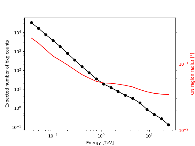
We add some control plots showing the expected number of background counts per bin and the ON region size cut (here the 68% containment radius of the PSF).
Plot expected number of counts for signal and background.
fig, ax1 = plt.subplots()
ax1.plot(
    sensitivity_table["e_ref"],
    sensitivity_table["background"],
    "o-",
    color="black",
    label="background",
)

ax1.loglog()
ax1.set_xlabel(f"Energy [{t['e_ref'].unit.to_string(UNIT_STRING_FORMAT)}]")
ax1.set_ylabel("Expected number of bkg counts")

ax2 = ax1.twinx()
ax2.set_ylabel(
    f"ON region radius [{on_radii.unit.to_string(UNIT_STRING_FORMAT)}]", color="red"
)
ax2.semilogy(sensitivity_table["e_ref"], on_radii, color="red", label="PSF68")
ax2.tick_params(axis="y", labelcolor="red")
ax2.set_ylim(0.01, 0.5)
plt.show()
Obtaining an integral flux sensitivity#
It is often useful to obtain the integral sensitivity above a certain threshold. In this case, it is simplest to use a dataset with one energy bin while setting the high energy edge to a very large value. Here, we simply squash the previously created dataset into one with a single energy
dataset_on_off1 = dataset_on_off.to_image()
sensitivity_estimator = SensitivityEstimator(
    gamma_min=5, n_sigma=3, bkg_syst_fraction=0.10
)
sensitivity_table = sensitivity_estimator.run(dataset_on_off1)
print(sensitivity_table)
 e_ref   e_min e_max     e2dnde     excess background criterion
  TeV     TeV   TeV  erg / (s cm2)
-------- ----- ----- ------------- ------- ---------- ---------
0.948683  0.03    30   1.44749e-12 6390.29    63902.9       bkg
To get the integral flux, we convert to a FluxPoints object
that does the conversion internally.
flux_points = FluxPoints.from_table(
    sensitivity_table,
    sed_type="e2dnde",
    reference_model=sensitivity_estimator.spectral_model,
)
print(
    f"Integral sensitivity in {livetime:.2f} above {energy_axis.edges[0]:.2e} "
    f"is {np.squeeze(flux_points.flux.quantity):.2e}"
)
Integral sensitivity in 50.00 h above 3.00e-02 TeV is 3.01e-11 1 / (s cm2)
Exercises#
Compute the sensitivity for a 20 hour observation
Compare how the sensitivity differs between 5 and 20 hours by plotting the ratio as a function of energy.