Modeling and Fitting (DL4 to DL5)#
Modeling#
gammapy.modeling contains all the functionalities related to modeling and fitting
data. This includes spectral, spatial and temporal model classes, as well as the fit
and parameter API.
Assuming you have prepared your gamma-ray data as a set of Dataset objects, and
stored one or more datasets in a Datasets container, you are all set for modeling
and fitting. Either via a YAML config file, or via Python code, define the
Models to use, which is a list of SkyModel objects
representing additive emission components, usually sources or diffuse emission, although a single source
can also be modeled by multiple components if you want. The SkyModel is a
factorised model with a SpectralModel component, a
SpatialModel component and a TemporalModel,
depending of the type of Datasets.
Most commonly used models in gamma-ray astronomy are built-in, see the Model gallery. It is easy to sum models, create compound spectral models (see Compound spectral model), or to create user-defined models (see Implementing a custom model). Gammapy is very flexible!
Models can be unique for a given dataset, or contribute to multiple datasets and thus provide links, allowing e.g. to do a joint fit to multiple IACT datasets, or to a joint IACT and Fermi-LAT dataset (see Multi instrument joint 3D and 1D analysis).
Built-in models#
Gammapy provides a large choice of spatial, spectral and temporal models. You may check out the whole list of built-in models in the Model gallery.
Custom models#
Gammapy provides an easy interface to Implementing a custom model.
Using gammapy.modeling#
Fitting#
Gammapy offers several statistical methods to estimate ‘best’ parameters from the data:
Maximum Likelihood Estimation (MLE)
Maximum A Posteriori estimation (MAP)
Bayesian Inference
Maximum Likelihood Estimation (MLE)#
This method permits to estimate parameters without having some knowledge on their probability distribution. Their “prior” distributions are then uniform in the region of interest. The estimation is achieved by maximizing a likelihood function by finding the models’ parameters for which the observed data have the highest joint probability. For this method, the “probability” is equivalent to “frequency”. It is a Frequentist inference of parameters from sample-data, permitting hypothesis testing, confidence intervals and confidence limits. Commonly, this method is a “fit” on the data.
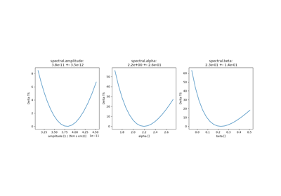
The Fit class provides methods to fit, i.e. optimise parameters and estimate parameter
errors and correlations. It interfaces with a Datasets object, which in turn is
connected to a Models object, which has a Parameters
object, which contains the model parameters.
Three different fitting backend are offered:
Sherpa is not installed by default, but this is quite easy (see Recommended Setup).
The tutorial Fitting describes in detail the API.
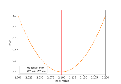
Maximum A Posteriori estimation (MAP)#
For some physics use cases, some parameters of the models might have some astrophysical constraints, e.g.
the usual case of positive flux, spectral index range. These knowledge can be used when estimating
parameters. To do so, we incorporate a Prior density over the quantities
one wants to estimate and the Fit class is used to determine the best parameters by
by regularizing the maximum a posteriori likelihood (a combination of the data likelihood term and of the prior
term).
With the MAP estimation, one can also realise hypothesis testing, compute confidence intervals and confidence limits.
The tutorial Priors describes in detail this estimation method.
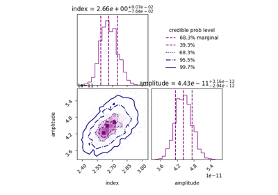
Bayesian Inference#
This Bayesian method uses prior knowledge on each models’ parameters, as Prior,
in order to estimate the posterior probabilities for each set of parameters values. They are
traditionally visualised in the form of corner plots of the parameters. This inference of the best
a posteriori parameters are not associated to the “best model” in the Frequentist sense, but rather to
the most probable given a set of parameters’ priors.
The Bayesian Inference is using dedicated tools to estimate posterior likelihood probabilities, e.g. the Markov Chain Monte Carlo (MCMC) approach or the Nested sampling (NS) approach that we recommend for Gammapy.
This method is quite powerful in case of non-Gaussian degeneracies, larger number of parameters, or to
map likelihood landscapes with multiple solutions (local maxima in which a classical fit would fall into).
However, the computation time to make Bayesian Inference is generally larger than for the Maximum
Likelihood Estimation using iminuit.
The tutorial Bayesian analysis with nested sampling describes in detail this estimation method.