estimators - High level estimators
Introduction
The gammapy.estimators submodule contains algorithms and classes
for high level flux and significance estimation. This includes
estimation flux points, flux maps, flux points, flux profiles and
flux light curves. All estimators feature a common API and allow
to estimate fluxes in bands of reconstructed energy.
The core of any estimator algorithm is hypothesis testing: a reference model or counts excess is tested against a null hypothesis. From the best fit reference model a flux is derived and a corresponding \(\Delta TS\) value from the difference in fit statistics to the null hypothesis. Assuming one degree of freedom, \(\sqrt{\Delta TS}\) represents an approximation (Wilk’s theorem) of the “classical significance”. In case of a negative best fit flux, e.g. when the background is overestimated, the significance is defined as \(-\sqrt{\Delta TS}\) by convention.
In general the flux can be estimated using two methods:
Based on model fitting: given a (global) best fit model with multiple model components, the flux of the component of interest is re-fitted in the chosen energy, time or spatial region. The new flux is given as a
normwith respect to the global reference model. Optionally other component parameters in the global model can be re-optimised. This method is also named forward folding.Based on excess: in the case of having one energy bin, neglecting the PSF and not re-optimising other parameters, one can estimate the significance based on the analytical solution by [LiMa1983]. In this case the “best fit” flux and significance are given by the excess over the null hypothesis. This method is also named backward folding. This method is currently only exposed in the
ExcessMapEstimator
In case the data is fitted to a single data bin only, e.g. one energy bin Uniformly for both methods most estimators compute the same basic quantities:
Quantity |
Definition |
|---|---|
norm |
Best fit norm with respect to the reference spectral model |
norm_err |
Symmetric error on the norm derived from the Hessian matrix |
stat |
Fit statistics value of the best fit hypothesis |
stat_null |
Fit statistics value of the null hypothesis |
ts |
Difference in fit statistics ( |
sqrt_ts |
Square root of ts time sign(norm), in case of one degree of freedom, corresponds to significance (Wilk’s theorem) |
npred |
Predicted counts of the best fit hypothesis. Equivalent to correlated counts for backward folding |
npred_excess |
Predicted excess counts of the best fit hypothesis. Equivalent to correlated excess for backward folding |
npred_background |
Predicted background counts of the best fit hypothesis. Equivalent to correlated excess for backward folding |
In addition the following optional quantities can be computed:
Quantity |
Definition |
|---|---|
norm_errp |
Positive error of the norm |
norm_errn |
Negative error of the norm |
norm_ul |
Upper limit of the norm |
norm_scan |
Norm scan |
stat_scan |
Fit statistics scan |
To compute the error, asymmetric errors as well as upper limits one can
specify the arguments n_sigma and n_sigma_ul. The n_sigma
arguments are translated into a TS difference assuming ts = n_sigma ** 2.
In addition to the norm values a reference spectral model and energy ranges are given. Using this reference spectral model the norm values can be converted to the following different SED types:
Quantity |
Definition |
|---|---|
e_ref |
Reference energy |
e_min |
Minimum energy |
e_max |
Maximum energy |
dnde |
Differential flux at |
flux |
Integrated flux between |
eflux |
Integrated energy flux between |
e2dnde |
Differential energy flux between |
The same can be applied for the error and upper limit information. More information can be found on the likelihood SED type page.
The FluxPoints and FluxMaps objects can optionally define meta
data with the following valid keywords:
Name |
Definition |
|---|---|
n_sigma |
Number of sigma used for error estimation |
n_sigma_ul |
Number of sigma used for upper limit estimation |
ts_threshold_ul |
TS threshold to define the use of an upper limit |
A note on negative flux and upper limit values:
Note
Gammapy allows for negative flux values and upper limits by default. While those values are physically not valid solutions, they are still valid statistically. Negative flux values either hint at overestimated background levels or underestimated systematic errors in general. Or in case of many measurements, such as pixels in a flux map, they are even statistically expected. For flux points and light curves the amplitude limits (if defined) are taken into account. In future versions of Gammapy it will be possible to account for systematic errors in the likelihood as well. For now the correct interpretation of the results is left to the user.
Getting started
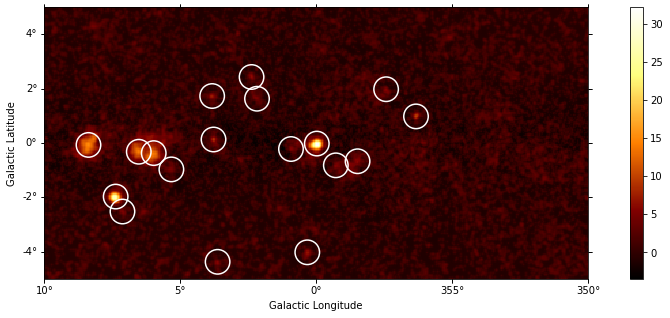
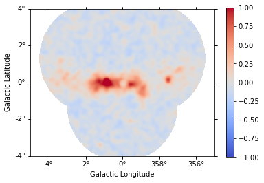
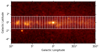
Flux maps
This how to compute flux maps with the ExcessMapEstimator:
import numpy as np
from gammapy.datasets import MapDataset
from gammapy.estimators import ExcessMapEstimator
from astropy import units as u

dataset = MapDataset.read("$GAMMAPY_DATA/cta-1dc-gc/cta-1dc-gc.fits.gz")

estimator = ExcessMapEstimator(
    correlation_radius="0.1 deg", energy_edges=[0.1, 1, 10] * u.TeV
)

maps = estimator.run(dataset)
print(maps["flux"])
WcsNDMap
<BLANKLINE>
    geom  : WcsGeom
    axes  : ['lon', 'lat', 'energy']
    shape : (320, 240, 2)
    ndim  : 3
    unit  : 1 / (cm2 s)
    dtype : float64
<BLANKLINE>
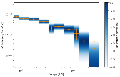
Flux points
This is how to compute flux points:
from astropy import units as u
from gammapy.datasets import SpectrumDatasetOnOff, Datasets
from gammapy.estimators import FluxPointsEstimator
from gammapy.modeling.models import PowerLawSpectralModel, SkyModel

path = "$GAMMAPY_DATA/joint-crab/spectra/hess/"
dataset_1 = SpectrumDatasetOnOff.read(path + "pha_obs23523.fits")
dataset_2 = SpectrumDatasetOnOff.read(path + "pha_obs23592.fits")

datasets = Datasets([dataset_1, dataset_2])

pwl = PowerLawSpectralModel(index=2, amplitude='1e-12  cm-2 s-1 TeV-1')

datasets.models = SkyModel(spectral_model=pwl, name="crab")

estimator = FluxPointsEstimator(
    source="crab", energy_edges=[0.1, 0.3, 1, 3, 10, 30, 100] * u.TeV
)

# this will run a joint fit of the datasets
fp = estimator.run(datasets)
table = fp.to_table(sed_type="dnde", formatted=True)
# print(table[["e_ref", "dnde", "dnde_err"]])

# or stack the datasets
# fp = estimator.run(datasets.stack_reduce())
table = fp.to_table(sed_type="dnde", formatted=True)
# print(table[["e_ref", "dnde", "dnde_err"]])
Reference/API
gammapy.estimators Package
Estimators.
Classes
|
Flux points container. |
|
A flux map / points container. |
Abstract estimator base class. |
|
|
Computes correlated excess, significance and error maps from a map dataset. |
|
Compute TS map from a MapDataset using different optimization methods. |
|
Flux points estimator. |
|
Adaptively smooth counts image. |
|
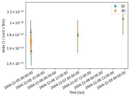
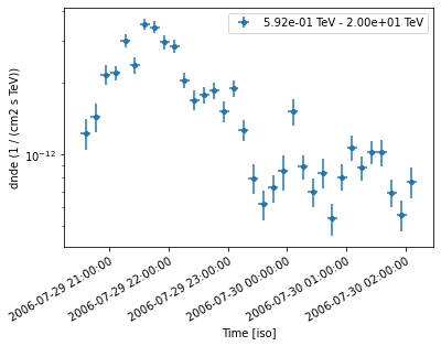
Estimate light curve. |
|
Estimate differential sensitivity. |
|
Estimate flux profiles |
Variables
Registry of estimator classes in Gammapy. |