Gaussian spatial model

This is a spatial model parametrising a Gaussian function.

By default, the Gaussian is symmetric:

\[\phi(\text{lon}, \text{lat}) = N \times \exp\left\{-\frac{1}{2} \frac{1-\cos \theta}{1-\cos \sigma}\right\}\,,\]

where \(\theta\) is the sky separation to the model center. In this case, the Gaussian is normalized to 1 on the sphere:

\[N = \frac{1}{4\pi a\left[1-\exp(-1/a)\right]}\,,\,\,\,\, a = 1-\cos \sigma\,.\]

In the limit of small \(\theta\) and \(\sigma\), this definition reduces to the usual form:

\[\phi(\text{lon}, \text{lat}) = \frac{1}{2\pi\sigma^2} \exp{\left(-\frac{1}{2} \frac{\theta^2}{\sigma^2}\right)}\,.\]

In case an eccentricity (\(e\)) and rotation angle (\(\phi\)) are passed, then the model is an elongated Gaussian, whose evaluation is performed as in the symmetric case but using the effective radius of the Gaussian:

\[\sigma_{eff}(\text{lon}, \text{lat}) = \sqrt{ (\sigma_M \sin(\Delta \phi))^2 + (\sigma_m \cos(\Delta \phi))^2 }.\]

Here, \(\sigma_M\) (\(\sigma_m\)) is the major (minor) semiaxis of the Gaussian, and \(\Delta \phi\) is the difference between phi, the position angle of the Gaussian, and the position angle of the evaluation point.

Caveat: For the asymmetric Gaussian, the model is normalized to 1 on the plane, i.e. in small angle approximation: \(N = 1/(2 \pi \sigma_M \sigma_m)\). This means that for huge elongated Gaussians on the sky this model is not correctly normalized. However, this approximation is perfectly acceptable for the more common case of models with modest dimensions: indeed, the error introduced by normalizing on the plane rather than on the sphere is below 0.1% for Gaussians with radii smaller than ~ 5 deg.

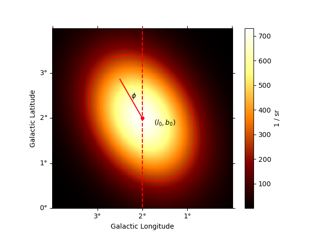
Example plot

Here is an example plot of the model:

import numpy as np
from astropy.coordinates import Angle
from gammapy.maps import WcsGeom
from gammapy.modeling.models import (
    GaussianSpatialModel,
    Models,
    PowerLawSpectralModel,
    SkyModel,
)

phi = Angle("30 deg")
model = GaussianSpatialModel(
    lon_0="2 deg",
    lat_0="2 deg",
    sigma="1 deg",
    e=0.7,
    phi=phi,
    frame="galactic",
)

geom = WcsGeom.create(
    skydir=model.position, frame=model.frame, width=(4, 4), binsz=0.02
)
ax = model.plot(geom=geom, add_cbar=True)

# illustrate size parameter
region = model.to_region().to_pixel(ax.wcs)
artist = region.as_artist(facecolor="none", edgecolor="red")
ax.add_artist(artist)

transform = ax.get_transform("galactic")
ax.scatter(2, 2, transform=transform, s=20, edgecolor="red", facecolor="red")
ax.text(1.5, 1.85, r"$(l_0, b_0)$", transform=transform, ha="center")
ax.plot([2, 2 + np.sin(phi)], [2, 2 + np.cos(phi)], color="r", transform=transform)
ax.vlines(x=2, color="r", linestyle="--", transform=transform, ymin=-5, ymax=5)
ax.text(2.25, 2.45, r"$\phi$", transform=transform)

YAML representation

Here is an example YAML file using the model:

pwl = PowerLawSpectralModel()
gauss = GaussianSpatialModel()

model = SkyModel(spectral_model=pwl, spatial_model=gauss, name="pwl-gauss-model")
models = Models([model])

print(models.to_yaml())

Out:

components:
-   name: pwl-gauss-model
    type: SkyModel
    spectral:
        type: PowerLawSpectralModel
        parameters:
        -   name: index
            value: 2.0
        -   name: amplitude
            value: 1.0e-12
            unit: cm-2 s-1 TeV-1
        -   name: reference
            value: 1.0
            unit: TeV
            frozen: true
    spatial:
        type: GaussianSpatialModel
        frame: icrs
        parameters:
        -   name: lon_0
            value: 0.0
            unit: deg
        -   name: lat_0
            value: 0.0
            unit: deg
        -   name: sigma
            value: 1.0
            unit: deg
        -   name: e
            value: 0.0
            frozen: true
        -   name: phi
            value: 0.0
            unit: deg
            frozen: true