This is a fixed-text formatted version of a Jupyter notebook
Try online

You may download all the notebooks in the documentation as a tar file.
Source files: overview.ipynb | overview.py
Data structures
Introduction
This is a getting started tutorial for Gammapy.
In this tutorial we will use the Second Fermi-LAT Catalog of High-Energy Sources (3FHL) catalog, corresponding event list and images to learn how to work with some of the central Gammapy data structures.
We will cover the following topics:
Sky maps
We will learn how to handle image based data with gammapy using a Fermi-LAT 3FHL example image. We will work with the following classes:
Event lists
We will learn how to handle event lists with Gammapy. Important for this are the following classes:
Source catalogs
We will show how to load source catalogs with Gammapy and explore the data using the following classes:
Spectral models and flux points
We will pick an example source and show how to plot its spectral model and flux points. For this we will use the following classes:
Setup
Important: to run this tutorial the environment variable GAMMAPY_DATA must be defined and point to the directory on your machine where the datasets needed are placed. To check whether your setup is correct you can execute the following cell:
[1]:
import os

path = os.path.expandvars("$GAMMAPY_DATA")

if not os.path.exists(path):
    raise Exception("gammapy-data repository not found!")
else:
    print("Great your setup is correct!")
Great your setup is correct!
In case you encounter an error, you can un-comment and execute the following cell to continue. But we recommend to set up your environment correctly as described here after you are done with this notebook.
[2]:
# os.environ['GAMMAPY_DATA'] = os.path.join(os.getcwd(), '..')
Now we can continue with the usual IPython notebooks and Python imports:
[3]:
%matplotlib inline
import matplotlib.pyplot as plt
[4]:
import astropy.units as u
from astropy.coordinates import SkyCoord
Maps
The gammapy.maps package contains classes to work with sky images and cubes.
In this section, we will use a simple 2D sky image and will learn how to:
Read sky images from FITS files
Smooth images
Plot images
Cutout parts from images
[5]:
from gammapy.maps import Map
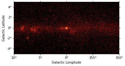
gc_3fhl = Map.read("$GAMMAPY_DATA/fermi-3fhl-gc/fermi-3fhl-gc-counts.fits.gz")
The image is a gammapy.maps.WcsNDMap object:
[6]:
gc_3fhl
[6]:
WcsNDMap

        geom  : WcsGeom
        axes  : ['lon', 'lat']
        shape : (400, 200)
        ndim  : 2
        unit  :
        dtype : >i8
The shape of the image is 400 x 200 pixel and it is defined using a cartesian projection in galactic coordinates.
The geom attribute is a gammapy.maps.WcsGeom object:
[7]:
gc_3fhl.geom
[7]:
WcsGeom

        axes       : ['lon', 'lat']
        shape      : (400, 200)
        ndim       : 2
        frame      : galactic
        projection : CAR
        center     : 0.0 deg, 0.0 deg
        width      : 20.0 deg x 10.0 deg
        wcs ref    : 0.0 deg, 0.0 deg
Let’s take a closer look a the .data attribute:
[8]:
gc_3fhl.data
[8]:
array([[0, 0, 0, ..., 0, 0, 0],
       [0, 0, 0, ..., 0, 0, 0],
       [0, 0, 0, ..., 0, 0, 0],
       ...,
       [0, 0, 0, ..., 0, 0, 1],
       [0, 0, 0, ..., 0, 0, 0],
       [0, 0, 0, ..., 0, 0, 1]])
That looks familiar! It just an ordinary 2 dimensional numpy array, which means you can apply any known numpy method to it:
[9]:
print(f"Total number of counts in the image: {gc_3fhl.data.sum():.0f}")
Total number of counts in the image: 32684
To show the image on the screen we can use the plot method. It basically calls plt.imshow, passing the gc_3fhl.data attribute but in addition handles axis with world coordinates using astropy.visualization.wcsaxes and defines some defaults for nicer plots (e.g. the colormap ‘afmhot’):
[10]:
gc_3fhl.plot(stretch="sqrt");
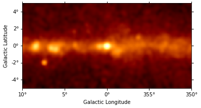
To make the structures in the image more visible we will smooth the data using a Gaussian kernel.
[11]:
gc_3fhl_smoothed = gc_3fhl.smooth(kernel="gauss", width=0.2 * u.deg)
[12]:
gc_3fhl_smoothed.plot(stretch="sqrt");
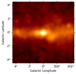
The smoothed plot already looks much nicer, but still the image is rather large. As we are mostly interested in the inner part of the image, we will cut out a quadratic region of the size 9 deg x 9 deg around Vela. Therefore we use gammapy.maps.Map.cutout to make a cutout map:
[13]:
# define center and size of the cutout region
center = SkyCoord(0, 0, unit="deg", frame="galactic")
gc_3fhl_cutout = gc_3fhl_smoothed.cutout(center, 9 * u.deg)
gc_3fhl_cutout.plot(stretch="sqrt");
For a more detailed introduction to gammapy.maps, take a look a the maps.ipynb notebook.
Exercises
Add a marker and circle at the position of
Sag A*(you can find examples in astropy.visualization.wcsaxes).
[ ]:
Event lists
Almost any high level gamma-ray data analysis starts with the raw measured counts data, which is stored in event lists. In Gammapy event lists are represented by the gammapy.data.EventList class.
In this section we will learn how to:
Read event lists from FITS files
Access and work with the
EventListattributes such as.tableand.energyFilter events lists using convenience methods
Let’s start with the import from the gammapy.data submodule:
[14]:
from gammapy.data import EventList
Very similar to the sky map class an event list can be created, by passing a filename to the gammapy.data.EventList.read() method:
[15]:
events_3fhl = EventList.read(
    "$GAMMAPY_DATA/fermi-3fhl-gc/fermi-3fhl-gc-events.fits.gz"
)
This time the actual data is stored as an astropy.table.Table object. It can be accessed with .table attribute:
[16]:
events_3fhl.table
[16]:
| ENERGY | RA | DEC | L | B | THETA | PHI | ZENITH_ANGLE | EARTH_AZIMUTH_ANGLE | TIME | EVENT_ID | RUN_ID | RECON_VERSION | CALIB_VERSION [3] | EVENT_CLASS [32] | EVENT_TYPE [32] | CONVERSION_TYPE | LIVETIME | DIFRSP0 | DIFRSP1 | DIFRSP2 | DIFRSP3 | DIFRSP4 |
|---|---|---|---|---|---|---|---|---|---|---|---|---|---|---|---|---|---|---|---|---|---|---|
| MeV | deg | deg | deg | deg | deg | deg | deg | deg | s | s | ||||||||||||
| float32 | float32 | float32 | float32 | float32 | float32 | float32 | float32 | float32 | float64 | int32 | int32 | int16 | int16 | bool | bool | int16 | float64 | float32 | float32 | float32 | float32 | float32 |
| 12186.642 | 260.45935 | -33.553337 | 353.36273 | 1.7538676 | 71.977325 | 125.50694 | 59.22307 | 231.79672 | 239572401.29222104 | 1823040 | 239571670 | 0 | 0 .. 0 | False .. True | False .. True | 0 | 238.57837238907814 | 0.0 | 0.0 | 0.0 | 0.0 | 0.0 |
| 25496.598 | 261.37506 | -34.395004 | 353.09607 | 0.6520652 | 42.49406 | 278.49347 | 41.092773 | 227.89838 | 239577842.16217342 | 550833 | 239577663 | 0 | 0 .. 0 | False .. True | False .. False | 1 | 176.16850754618645 | 0.0 | 0.0 | 0.0 | 0.0 | 0.0 |
| 15621.498 | 259.56973 | -33.409416 | 353.05673 | 2.4450684 | 64.32412 | 234.22194 | 66.526794 | 232.75734 | 239578244.7997108 | 1353175 | 239577663 | 0 | 0 .. 0 | False .. True | False .. False | 1 | 9.392075657844543 | 0.0 | 0.0 | 0.0 | 0.0 | 0.0 |
| 12816.32 | 273.95883 | -25.340391 | 6.45856 | -4.0548873 | 43.292503 | 142.87392 | 13.232716 | 108.02273 | 239605914.66160735 | 9636241 | 239601276 | 0 | 0 .. 0 | False .. True | False .. False | 1 | 4.034786552190781 | 0.0 | 0.0 | 0.0 | 0.0 | 0.0 |
| 18988.387 | 260.8568 | -36.355804 | 351.23734 | -0.101912394 | 26.916113 | 290.39337 | 23.8726 | 212.91147 | 239611913.14460415 | 11233188 | 239606871 | 0 | 0 .. 0 | False .. True | False .. True | 0 | 131.60132896900177 | 0.0 | 0.0 | 0.0 | 0.0 | 0.0 |
| 11610.23 | 266.15518 | -26.224436 | 2.1986027 | 1.6034819 | 35.77363 | 274.53387 | 23.537594 | 232.64166 | 239623554.55414733 | 14156811 | 239618329 | 0 | 0 .. 0 | False .. True | False .. False | 1 | 74.98110938072205 | 0.0 | 0.0 | 0.0 | 0.0 | 0.0 |
| 13960.802 | 271.44742 | -29.615316 | 1.6267247 | -4.1431155 | 25.917883 | 238.0368 | 15.037035 | 123.32094 | 239634549.1748726 | 14140569 | 239629788 | 0 | 0 .. 0 | False .. True | False .. False | 1 | 106.37336817383766 | 0.0 | 0.0 | 0.0 | 0.0 | 0.0 |
| 10477.372 | 266.3981 | -28.96814 | 359.97003 | -0.011748177 | 39.091587 | 275.5457 | 33.02354 | 229.59308 | 239635161.87982982 | 15688393 | 239629788 | 0 | 0 .. 0 | False .. True | False .. True | 0 | 214.62817406654358 | 0.0 | 0.0 | 0.0 | 0.0 | 0.0 |
| 13030.88 | 271.70428 | -20.632627 | 9.59348 | 0.026241468 | 52.622505 | 161.3205 | 39.350845 | 91.9986 | 239639873.2076075 | 1736482 | 239639436 | 0 | 0 .. 0 | False .. True | False .. True | 0 | 94.68753063678741 | 0.0 | 0.0 | 0.0 | 0.0 | 0.0 |
| 11517.904 | 265.00894 | -30.065119 | 358.40112 | 0.43904436 | 41.812317 | 276.02448 | 37.975704 | 229.18602 | 239652422.2848442 | 2116817 | 239651660 | 0 | 0 .. 0 | False .. True | False .. True | 0 | 123.15007302165031 | 0.0 | 0.0 | 0.0 | 0.0 | 0.0 |
| 19958.182 | 263.31854 | -37.094856 | 351.71606 | -2.153713 | 52.544586 | 121.415764 | 19.790777 | 195.32071 | 239657693.0997924 | 114586 | 239657673 | 0 | 0 .. 0 | False .. True | False .. True | 0 | 17.113530546426773 | 0.0 | 0.0 | 0.0 | 0.0 | 0.0 |
| 23760.14 | 265.4694 | -31.55994 | 357.34256 | -0.68805 | 52.70319 | 248.87813 | 53.087788 | 229.58832 | 239669871.23729014 | 577193 | 239669643 | 0 | 0 .. 0 | False .. True | False .. False | 1 | 225.2544113099575 | 0.0 | 0.0 | 0.0 | 0.0 | 0.0 |
| 32168.988 | 266.35397 | -30.096745 | 358.98682 | -0.56723064 | 64.830696 | 212.93645 | 67.121216 | 114.544685 | 239673726.5025267 | 7589046 | 239669643 | 0 | 0 .. 0 | False .. True | False .. False | 1 | 45.64776709675789 | 0.0 | 0.0 | 0.0 | 0.0 | 0.0 |
| 10165.9 | 266.15427 | -19.829279 | 7.668937 | 4.9320326 | 51.85829 | 207.0177 | 50.963444 | 95.7839 | 239691232.08568192 | 8295557 | 239687124 | 0 | 0 .. 0 | False .. True | False .. True | 0 | 204.40402576327324 | 0.0 | 0.0 | 0.0 | 0.0 | 0.0 |
| 25277.545 | 269.68344 | -24.668644 | 5.1628966 | -0.34179303 | 42.77833 | 129.13857 | 10.365034 | 205.91513 | 239697927.85482475 | 11566661 | 239692809 | 0 | 0 .. 0 | False .. True | False .. True | 0 | 85.29761010408401 | 0.0 | 0.0 | 0.0 | 0.0 | 0.0 |
| 223713.7 | 261.1885 | -31.794796 | 355.1619 | 2.239802 | 25.89418 | 284.8728 | 17.017782 | 206.84254 | 239703590.65764225 | 12808348 | 239698539 | 0 | 0 .. 0 | False .. True | False .. True | 0 | 166.99824661016464 | 0.0 | 0.0 | 0.0 | 0.0 | 0.0 |
| 15236.758 | 264.52255 | -31.730831 | 356.7694 | -0.09604572 | 51.646976 | 141.44576 | 24.359364 | 113.722145 | 239708834.38999206 | 12626484 | 239704268 | 0 | 0 .. 0 | False .. True | False .. True | 0 | 5.334206968545914 | 0.0 | 0.0 | 0.0 | 0.0 | 0.0 |
| 36314.297 | 264.79855 | -31.116806 | 357.41434 | 0.032732587 | 48.567314 | 122.824875 | 17.206326 | 204.58994 | 239709375.13045236 | 14186184 | 239704268 | 0 | 0 .. 0 | False .. True | False .. False | 1 | 34.09180650115013 | 0.0 | 0.0 | 0.0 | 0.0 | 0.0 |
| ... | ... | ... | ... | ... | ... | ... | ... | ... | ... | ... | ... | ... | ... | ... | ... | ... | ... | ... | ... | ... | ... | ... |
| 74033.305 | 268.76508 | -24.43612 | 4.944724 | 0.4974049 | 51.1174 | 225.20499 | 1.1782029 | 344.13354 | 459968408.4067848 | 3353048 | 459967402 | 0 | 0 .. 0 | False .. True | False .. True | 0 | 65.83160126209259 | 0.0 | 0.0 | 0.0 | 0.0 | 0.0 |
| 47114.324 | 266.99127 | -28.421051 | 0.70769924 | -0.1726071 | 60.81272 | 212.27025 | 45.926052 | 112.289925 | 460036242.88448673 | 7874108 | 460032656 | 0 | 0 .. 0 | False .. True | False .. False | 1 | 77.02012866735458 | 0.0 | 0.0 | 0.0 | 0.0 | 0.0 |
| 14473.36 | 259.55792 | -32.497227 | 353.79837 | 2.9774146 | 69.47437 | 136.79776 | 46.463108 | 120.018074 | 460030422.7761504 | 6834438 | 460026946 | 0 | 0 .. 0 | False .. True | False .. True | 0 | 13.922565162181854 | 0.0 | 0.0 | 0.0 | 0.0 | 0.0 |
| 20056.527 | 267.50372 | -21.494694 | 6.888726 | 2.9924572 | 46.228405 | 129.99919 | 6.3767605 | 305.91837 | 460031341.48834544 | 9754178 | 460026946 | 0 | 0 .. 0 | False .. True | False .. False | 1 | 115.29787397384644 | 0.0 | 0.0 | 0.0 | 0.0 | 0.0 |
| 10021.135 | 266.58603 | -29.006046 | 0.023192262 | -0.17183326 | 58.983257 | 139.42741 | 29.243576 | 109.29137 | 460042219.35562307 | 9552550 | 460038366 | 0 | 0 .. 0 | False .. True | False .. True | 0 | 115.27116513252258 | 0.0 | 0.0 | 0.0 | 0.0 | 0.0 |
| 11217.242 | 260.67258 | -32.080307 | 354.67896 | 2.4407566 | 76.96116 | 214.30273 | 77.80194 | 121.61477 | 460104239.29869664 | 5218298 | 460101374 | 0 | 0 .. 0 | False .. True | False .. False | 1 | 64.04110872745514 | 0.0 | 0.0 | 0.0 | 0.0 | 0.0 |
| 18494.64 | 267.2745 | -36.705185 | 353.7175 | -4.6370916 | 38.942596 | 226.92189 | 13.237086 | 149.41605 | 460116880.22025174 | 9578197 | 460112590 | 0 | 0 .. 0 | False .. True | False .. False | 1 | 111.12007641792297 | 0.0 | 0.0 | 0.0 | 0.0 | 0.0 |
| 13333.997 | 265.57535 | -31.519987 | 357.42413 | -0.7436878 | 43.89681 | 230.49913 | 7.34928 | 145.94727 | 460128338.6831755 | 11459159 | 460124010 | 0 | 0 .. 0 | False .. True | False .. False | 1 | 23.238793969154358 | 0.0 | 0.0 | 0.0 | 0.0 | 0.0 |
| 13160.466 | 269.90778 | -24.671898 | 5.2616706 | -0.52015543 | 60.9269 | 226.45708 | 40.456112 | 248.86581 | 460163408.5927998 | 114271 | 460163403 | 0 | 0 .. 0 | False .. True | False .. True | 0 | 1.9516496658325195 | 0.0 | 0.0 | 0.0 | 0.0 | 0.0 |
| 387834.72 | 270.3779 | -21.56711 | 8.171749 | 0.64531475 | 56.755512 | 221.84715 | 24.358454 | 86.67913 | 460185260.7970139 | 7595626 | 460181260 | 0 | 0 .. 0 | False .. True | False .. True | 0 | 34.214694023132324 | 0.0 | 0.0 | 0.0 | 0.0 | 0.0 |
| 20559.74 | 268.5538 | -26.345692 | 3.200638 | -0.30328986 | 49.523575 | 233.67285 | 12.370642 | 250.35716 | 460185803.2027966 | 8785590 | 460181260 | 0 | 0 .. 0 | False .. True | False .. True | 0 | 103.17629969120026 | 0.0 | 0.0 | 0.0 | 0.0 | 0.0 |
| 27209.146 | 266.59344 | -30.52607 | 358.72775 | -0.96718174 | 62.1856 | 140.27434 | 32.686306 | 109.74662 | 460190778.6372646 | 7274453 | 460186976 | 0 | 0 .. 0 | False .. True | False .. True | 0 | 43.22334712743759 | 0.0 | 0.0 | 0.0 | 0.0 | 0.0 |
| 13911.061 | 269.30997 | -27.239439 | 2.7684028 | -1.3365301 | 65.15399 | 224.52101 | 53.017742 | 242.62904 | 460197889.2652691 | 12049887 | 460192198 | 0 | 0 .. 0 | False .. True | False .. True | 0 | 95.46356403827667 | 0.0 | 0.0 | 0.0 | 0.0 | 0.0 |
| 13226.425 | 265.16287 | -27.344238 | 0.7796942 | 1.7680178 | 59.38332 | 126.7019 | 32.12299 | 246.97205 | 460203215.10816145 | 11716888 | 460198235 | 0 | 0 .. 0 | False .. True | False .. False | 1 | 3.733097553253174 | 0.0 | 0.0 | 0.0 | 0.0 | 0.0 |
| 17445.463 | 266.63342 | -28.807201 | 0.21464892 | -0.1039705 | 55.48627 | 135.59155 | 14.227151 | 106.7812 | 460225372.9842249 | 1679082 | 460224933 | 0 | 0 .. 0 | False .. True | False .. False | 1 | 80.52235281467438 | 0.0 | 0.0 | 0.0 | 0.0 | 0.0 |
| 13133.864 | 270.42474 | -22.651058 | 7.251185 | 0.071358204 | 48.704975 | 134.73102 | 2.489122 | 294.48605 | 460225688.52486295 | 2879335 | 460224933 | 0 | 0 .. 0 | False .. True | False .. False | 1 | 117.88173341751099 | 0.0 | 0.0 | 0.0 | 0.0 | 0.0 |
| 32095.705 | 266.0002 | -29.77206 | 359.1034 | -0.13615231 | 45.013103 | 236.72498 | 6.92107 | 212.86594 | 460231367.1387127 | 1113706 | 460231084 | 0 | 0 .. 0 | False .. True | False .. True | 0 | 108.92976492643356 | 0.0 | 0.0 | 0.0 | 0.0 | 0.0 |
| 18465.783 | 266.39728 | -29.105953 | 359.85202 | -0.08294058 | 55.97552 | 135.87787 | 18.909636 | 112.137924 | 459939497.057684 | 7689831 | 459935572 | 0 | 0 .. 0 | False .. True | False .. True | 0 | 70.72638684511185 | 0.0 | 0.0 | 0.0 | 0.0 | 0.0 |
| 14457.25 | 262.72217 | -34.388405 | 353.7184 | -0.26906812 | 45.683174 | 237.74162 | 25.728264 | 240.87035 | 459945845.4798405 | 10049680 | 459941302 | 0 | 0 .. 0 | False .. True | False .. True | 0 | 147.4274787902832 | 0.0 | 0.0 | 0.0 | 0.0 | 0.0 |
You can do len over event_3fhl.table to find the total number of events.
[17]:
len(events_3fhl.table)
[17]:
32843
And we can access any other attribute of the Table object as well:
[18]:
events_3fhl.table.colnames
[18]:
['ENERGY',
 'RA',
 'DEC',
 'L',
 'B',
 'THETA',
 'PHI',
 'ZENITH_ANGLE',
 'EARTH_AZIMUTH_ANGLE',
 'TIME',
 'EVENT_ID',
 'RUN_ID',
 'RECON_VERSION',
 'CALIB_VERSION',
 'EVENT_CLASS',
 'EVENT_TYPE',
 'CONVERSION_TYPE',
 'LIVETIME',
 'DIFRSP0',
 'DIFRSP1',
 'DIFRSP2',
 'DIFRSP3',
 'DIFRSP4']
For convenience we can access the most important event parameters as properties on the EventList objects. The attributes will return corresponding Astropy objects to represent the data, such as astropy.units.Quantity, astropy.coordinates.SkyCoord or
astropy.time.Time objects:
[19]:
events_3fhl.energy.to("GeV")
[19]:
[20]:
events_3fhl.galactic
# events_3fhl.radec
[20]:
<SkyCoord (Galactic): (l, b) in deg
    [(353.36228879,  1.75408483), (353.09562941,  0.6522806 ),
     (353.05628243,  2.44528685), ..., (359.10295505, -0.1359316 ),
     (359.85157506, -0.08269984), (353.71795506, -0.26883694)]>
[21]:
events_3fhl.time
[21]:
<Time object: scale='tt' format='mjd' value=[54682.82946153 54682.89243456 54682.89709472 ... 57236.75267735
 57233.37455141 57233.44802852]>
In addition EventList provides convenience methods to filter the event lists. One possible use case is to find the highest energy event within a radius of 0.5 deg around the vela position:
[22]:
# select all events within a radius of 0.5 deg around center
from gammapy.utils.regions import SphericalCircleSkyRegion

region = SphericalCircleSkyRegion(center, radius=0.5 * u.deg)
events_gc_3fhl = events_3fhl.select_region(region)

# sort events by energy
events_gc_3fhl.table.sort("ENERGY")

# and show highest energy photon
events_gc_3fhl.energy[-1].to("GeV")
[22]:
Exercises
Make a counts energy spectrum for the galactic center region, within a radius of 10 deg.
[ ]:
Source catalogs
Gammapy provides a convenient interface to access and work with catalog based data.
In this section we will learn how to:
Load builtins catalogs from
gammapy.catalogSort and index the underlying Astropy tables
Access data from individual sources
Let’s start with importing the 3FHL catalog object from the gammapy.catalog submodule:
[23]:
from gammapy.catalog import SourceCatalog3FHL
First we initialize the Fermi-LAT 3FHL catalog and directly take a look at the .table attribute:
[24]:
fermi_3fhl = SourceCatalog3FHL()
fermi_3fhl.table
[24]:
| Source_Name | RAJ2000 | DEJ2000 | GLON | GLAT | Conf_95_SemiMajor | Conf_95_SemiMinor | Conf_95_PosAng | ROI_num | Signif_Avg | Pivot_Energy | Flux_Density | Unc_Flux_Density | Flux | Unc_Flux | Energy_Flux | Unc_Energy_Flux | Signif_Curve | SpectrumType | Spectral_Index | Unc_Spectral_Index | beta | Unc_beta | PowerLaw_Index | Unc_PowerLaw_Index | Flux_Band [5] | Unc_Flux_Band [5,2] | nuFnu [5] | Sqrt_TS_Band [5] | Npred | HEP_Energy | HEP_Prob | Variability_BayesBlocks | Extended_Source_Name | ASSOC_GAM | TEVCAT_FLAG | ASSOC_TEV | CLASS | ASSOC1 | ASSOC2 | ASSOC_PROB_BAY | ASSOC_PROB_LR | Redshift | NuPeak_obs |
|---|---|---|---|---|---|---|---|---|---|---|---|---|---|---|---|---|---|---|---|---|---|---|---|---|---|---|---|---|---|---|---|---|---|---|---|---|---|---|---|---|---|---|---|
| deg | deg | deg | deg | deg | deg | deg | GeV | 1 / (cm2 GeV s) | 1 / (cm2 GeV s) | 1 / (cm2 s) | 1 / (cm2 s) | erg / (cm2 s) | erg / (cm2 s) | 1 / (cm2 s) | 1 / (cm2 s) | erg / (cm2 s) | GeV | Hz | |||||||||||||||||||||||||
| bytes18 | float32 | float32 | float32 | float32 | float32 | float32 | float32 | int16 | float32 | float32 | float32 | float32 | float32 | float32 | float32 | float32 | float32 | bytes11 | float32 | float32 | float32 | float32 | float32 | float32 | float32 | float32 | float32 | float32 | float32 | float32 | float32 | int16 | bytes18 | bytes18 | bytes1 | bytes21 | bytes7 | bytes26 | bytes26 | float32 | float32 | float32 | float32 |
| 3FHL J0001.2-0748 | 0.3107 | -7.8075 | 89.0094 | -67.3118 | 0.0424 | 0.0424 | -- | 64 | 5.362 | 23.73 | 5.3174e-13 | 2.0975e-13 | 2.9593e-11 | 1.1704e-11 | 1.6752e-12 | 1.0743e-12 | 1.02 | PowerLaw | 1.6724 | 0.8274 | 0.5916 | 0.7129 | 2.2226 | 0.4808 | 1.1127661e-11 .. 1.1422301e-22 | -6.0763976e-12 .. 6.529277e-12 | 3.533989e-13 .. 1.1789072e-22 | 3.1458344 .. 0.0 | 7.63 | 86.975 | 0.9964 | 1 | 3FGL J0001.2-0748 | N | bll | PMN J0001-0746 | 0.9974 | 0.9721 | -- | 306196370000000.0 | |||
| 3FHL J0001.9-4155 | 0.4849 | -41.9303 | 334.1216 | -72.0697 | 0.1018 | 0.1018 | -- | 429 | 5.638 | 28.42 | 5.4253e-13 | 1.6839e-13 | 4.3230e-11 | 1.3428e-11 | 3.4900e-12 | 1.8276e-12 | 0.45 | PowerLaw | 1.7819 | 0.4941 | 0.1187 | 0.2798 | 1.9418 | 0.3100 | 2.1003905e-11 .. 1.9287885e-18 | -8.032091e-12 .. 5.8594097e-12 | 6.7452245e-13 .. 2.078675e-18 | 4.899907 .. 0.0 | 12.51 | 266.625 | 0.9622 | 1 | 3FGL J0002.2-4152 | N | bcu | 1RXS J000135.5-415519 | 0.9960 | 0.0000 | -- | 6309576500000000.0 | |||
| 3FHL J0002.1-6728 | 0.5283 | -67.4825 | 310.0868 | -48.9549 | 0.0357 | 0.0357 | -- | 386 | 8.470 | 20.82 | 1.2062e-12 | 3.2106e-13 | 5.0093e-11 | 1.3349e-11 | 2.3058e-12 | 9.5580e-13 | 1.53 | PowerLaw | 1.8109 | 0.6260 | 0.7933 | 0.5956 | 2.4285 | 0.3710 | 2.4550664e-11 .. 1.9009976e-21 | -8.634195e-12 .. 4.8021903e-12 | 7.7340695e-13 .. 1.9026535e-21 | 5.900217 .. 0.0 | 17.11 | 52.152 | 0.9988 | 1 | 3FGL J0002.0-6722 | N | bcu | SUMSS J000215-672653 | 0.0000 | 0.9395 | -- | 4466832000000000.0 | |||
| 3FHL J0003.3-5248 | 0.8300 | -52.8150 | 318.9245 | -62.7936 | 0.0425 | 0.0425 | -- | 145 | 7.229 | 23.66 | 7.5065e-13 | 2.3102e-13 | 4.1560e-11 | 1.2839e-11 | 2.2874e-12 | 1.1145e-12 | 1.70 | PowerLaw | 1.6010 | 0.5644 | 0.9972 | 0.1721 | 2.2481 | 0.3732 | 2.0886386e-11 .. 7.5867555e-23 | -8.143967e-12 .. 5.31299e-12 | 6.6265456e-13 .. 7.800202e-23 | 5.298393 .. 0.0 | 13.02 | 67.310 | 0.9636 | 1 | 3FGL J0003.2-5246 | N | bcu | RBS 0006 | 0.9996 | 0.9716 | -- | 7.079464e+16 | |||
| 3FHL J0007.0+7303 | 1.7647 | 73.0560 | 119.6625 | 10.4666 | 0.0101 | 0.0101 | -- | 277 | 75.265 | 12.80 | 1.7436e-10 | 7.5950e-12 | 1.5308e-09 | 6.1341e-11 | 3.6785e-11 | 1.5973e-12 | 3.24 | LogParabola | 3.1751 | 0.2103 | 0.9021 | 0.2659 | 3.8315 | 0.1141 | 1.3514667e-09 .. 3.839895e-18 | -5.7581186e-11 .. 4.060418e-12 | 4.109739e-11 .. 2.9231144e-18 | 71.33829 .. 0.0 | 654.15 | 60.292 | 0.9972 | 1 | 3FGL J0007.0+7302 | E | CTA 1 | PSR | LAT PSR J0007+7303 | 1.0000 | 0.0000 | -- | -- | ||
| 3FHL J0007.9+4711 | 1.9931 | 47.1920 | 115.3093 | -15.0354 | 0.0196 | 0.0196 | -- | 302 | 17.774 | 17.19 | 5.9778e-12 | 8.7683e-13 | 1.5131e-10 | 2.2181e-11 | 5.1444e-12 | 1.0540e-12 | 0.56 | PowerLaw | 2.6783 | 0.4196 | 0.1696 | 0.3282 | 2.8588 | 0.2685 | 1.0582407e-10 .. 1.9819723e-16 | -1.7538379e-11 .. 4.823511e-12 | 3.278615e-12 .. 1.8668298e-16 | 15.209969 .. 0.0 | 50.95 | 68.152 | 0.9759 | 1 | 3FGL J0008.0+4713 | N | bll | MG4 J000800+4712 | 1.0000 | 0.9873 | 0.2800 | 2511884200000000.0 | |||
| 3FHL J0008.4-2339 | 2.1243 | -23.6514 | 50.2908 | -79.7021 | 0.0366 | 0.0366 | -- | 517 | 9.679 | 16.96 | 3.0610e-12 | 7.3475e-13 | 7.4602e-11 | 1.7896e-11 | 2.4733e-12 | 8.1716e-13 | 0.34 | PowerLaw | 2.7388 | 0.7145 | 0.1737 | 0.5618 | 2.9070 | 0.4520 | 5.804992e-11 .. 1.1117311e-20 | -1.4419374e-11 .. 6.10661e-12 | 1.7951775e-12 .. 1.0403958e-20 | 9.133706 .. 0.0 | 19.83 | 71.122 | 0.9968 | 1 | 3FGL J0008.6-2340 | N | bll | RBS 0016 | 0.9996 | 0.9673 | 0.1470 | 524807800000000.0 | |||
| 3FHL J0009.1+0628 | 2.2874 | 6.4814 | 104.4637 | -54.8669 | 0.0385 | 0.0385 | -- | 402 | 6.282 | 18.92 | 1.2691e-12 | 4.3696e-13 | 4.1597e-11 | 1.4317e-11 | 1.6903e-12 | 8.9372e-13 | 0.10 | PowerLaw | 2.5529 | 0.8363 | 0.0122 | 0.4477 | 2.5800 | 0.5391 | 2.4161059e-11 .. 6.6482124e-19 | -9.546595e-12 .. 6.287476e-12 | 7.566492e-13 .. 6.5095056e-19 | 4.678369 .. 0.0 | 10.95 | 12.256 | 0.9721 | 1 | 3FGL J0009.1+0630 | N | bll | CRATES J000903.95+062821.5 | 0.9993 | 0.9878 | -- | 663742400000000.0 | |||
| 3FHL J0009.4+5030 | 2.3504 | 50.5049 | 116.1257 | -11.8105 | 0.0176 | 0.0176 | -- | 302 | 22.402 | 17.04 | 9.8252e-12 | 1.3192e-12 | 2.2191e-10 | 2.6212e-11 | 8.7336e-12 | 1.2488e-12 | 3.15 | LogParabola | 1.4305 | 0.3505 | 0.7965 | 0.3072 | 2.3610 | 0.1611 | 1.16274e-10 .. 9.252794e-17 | -1.8225135e-11 .. 4.417993e-12 | 3.8564165e-12 .. 7.0436765e-17 | 15.780677 .. 0.0 | 78.50 | 72.762 | 0.9950 | 2 | 3FGL J0009.3+5030 | C | bll | NVSS J000922+503028 | 1.0000 | 0.9698 | -- | 1412536400000000.0 | |||
| 3FHL J0009.7-4319 | 2.4450 | -43.3195 | 327.7563 | -71.7445 | 0.0496 | 0.0496 | -- | 429 | 4.957 | 16.77 | 1.0257e-12 | 4.2463e-13 | 2.4189e-11 | 1.0008e-11 | 7.8730e-13 | 4.3643e-13 | 1.00 | PowerLaw | 2.2044 | 0.9640 | 0.9994 | 0.0609 | 2.9442 | 0.7655 | 1.4262526e-11 .. 1.124737e-17 | -6.5860017e-12 .. 5.5998656e-12 | 4.4044038e-13 .. 1.04738585e-17 | 4.1469994 .. 0.0 | 7.00 | 26.010 | 0.9912 | 1 | N | bll | SUMSS J000949-431654 | 0.9985 | 0.9072 | -- | -- | ||||
| 3FHL J0013.0-3956 | 3.2523 | -39.9381 | 332.3835 | -74.9150 | 0.0517 | 0.0517 | -- | 429 | 7.201 | 14.27 | 3.5994e-12 | 1.0357e-12 | 4.9878e-11 | 1.4376e-11 | 1.2946e-12 | 4.5911e-13 | 0.99 | PowerLaw | 3.0130 | 0.9492 | 0.9978 | 0.1128 | 3.6066 | 0.7866 | 4.1576055e-11 .. 4.364096e-18 | -1.1673498e-11 .. 5.6003054e-12 | 1.2527341e-12 .. 3.750808e-18 | 7.4368286 .. 0.0 | 14.19 | 20.627 | 0.9837 | 1 | 3FGL J0013.2-3954 | N | bll | PKS 0010-401 | 0.9998 | 0.9962 | -- | 1862089000000.0 | |||
| 3FHL J0013.8-1855 | 3.4684 | -18.9169 | 74.5314 | -78.0876 | 0.0485 | 0.0485 | -- | 152 | 5.272 | 18.94 | 9.4557e-13 | 3.6339e-13 | 3.1086e-11 | 1.1945e-11 | 1.2427e-12 | 7.0538e-13 | 1.06 | PowerLaw | 1.9438 | 0.9164 | 0.9135 | 0.8288 | 2.6020 | 0.5839 | 1.8761324e-11 .. 2.4010398e-18 | -8.03048e-12 .. 6.2478846e-12 | 5.8704425e-13 .. 2.343576e-18 | 4.4304204 .. 0.0 | 8.19 | 37.217 | 0.9861 | 1 | 3FGL J0013.9-1853 | P | SHBL J001355.9-185406 | bll | RBS 0030 | 0.9995 | 0.9772 | 0.0950 | 5.260181e+16 | ||
| 3FHL J0014.0-5024 | 3.5038 | -50.4003 | 317.4913 | -65.6568 | 0.0597 | 0.0597 | -- | 239 | 4.869 | 22.74 | 5.9817e-13 | 2.2478e-13 | 3.0263e-11 | 1.1370e-11 | 1.7404e-12 | 1.0928e-12 | 1.45 | PowerLaw | 1.4978 | 0.7488 | 0.9964 | 0.1776 | 2.2086 | 0.4499 | 1.0878415e-11 .. 1.7599409e-17 | -5.7917993e-12 .. 5.8792246e-12 | 3.4567488e-13 .. 1.8203253e-17 | 3.097385 .. 0.0 | 9.23 | 26.054 | 0.9927 | 1 | 3FGL J0014.0-5025 | N | bll | RBS 0032 | 0.9998 | 0.8923 | -- | 8.413936e+16 | |||
| 3FHL J0014.7+5801 | 3.6951 | 58.0244 | 118.0788 | -4.5015 | 0.0266 | 0.0266 | -- | 518 | 8.215 | 25.55 | 8.7309e-13 | 2.1415e-13 | 5.6736e-11 | 1.3982e-11 | 3.5097e-12 | 1.3787e-12 | 0.51 | PowerLaw | 2.0013 | 0.4443 | 0.1259 | 0.2631 | 2.1459 | 0.2768 | 3.2196253e-11 .. 6.0640007e-18 | -9.896842e-12 .. 4.293739e-12 | 1.0256123e-12 .. 6.3322123e-18 | 6.1053777 .. 0.0 | 22.02 | 160.817 | 0.9943 | 1 | 3FGL J0014.7+5802 | N | bll | 1RXS J001442.2+580201 | 1.0000 | 0.9778 | -- | 4.3651522e+16 | |||
| 3FHL J0014.9+6118 | 3.7366 | 61.3025 | 118.5645 | -1.2594 | 0.0339 | 0.0339 | -- | 518 | 9.091 | 15.86 | 4.2551e-12 | 8.4587e-13 | 8.4783e-11 | 1.6849e-11 | 2.5742e-12 | 6.9789e-13 | 0.00 | PowerLaw | 3.0910 | 0.5482 | 0.0089 | 0.4114 | 3.1010 | 0.4416 | 6.525263e-11 .. 2.2172363e-18 | -1.3828337e-11 .. 4.048499e-12 | 2.0031396e-12 .. 2.0232124e-18 | 8.736899 .. 0.0 | 33.68 | 34.407 | 0.9822 | 1 | 3FGL J0014.6+6119 | N | bcu | 4C +60.01 | 0.9994 | 0.9996 | -- | 12971790000000.0 | |||
| 3FHL J0015.7+5551 | 3.9337 | 55.8649 | 117.9031 | -6.6579 | 0.0335 | 0.0335 | -- | 302 | 8.112 | 31.18 | 5.5030e-13 | 1.3879e-13 | 5.2164e-11 | 1.3207e-11 | 4.5355e-12 | 1.9094e-12 | 0.74 | PowerLaw | 1.6969 | 0.3726 | 0.1531 | 0.2218 | 1.8898 | 0.2480 | 2.4335116e-11 .. 1.9521596e-17 | -8.442904e-12 .. 4.4789077e-12 | 7.8311885e-13 .. 2.1210226e-17 | 5.2631125 .. 0.0 | 19.71 | 167.578 | 0.9820 | 1 | 3FGL J0015.7+5552 | C | bll | GB6 J0015+5551 | 1.0000 | 0.9832 | -- | 6180169000000000.0 | |||
| 3FHL J0018.6+2946 | 4.6525 | 29.7821 | 114.4798 | -32.5503 | 0.0312 | 0.0312 | -- | 522 | 7.917 | 29.20 | 6.0010e-13 | 1.7106e-13 | 5.0577e-11 | 1.4495e-11 | 3.8639e-12 | 1.7982e-12 | 0.92 | PowerLaw | 1.6802 | 0.4901 | 0.2639 | 0.3270 | 1.9816 | 0.2912 | 2.3603335e-11 .. 0.0 | -9.441283e-12 .. 5.7002103e-12 | 7.568024e-13 .. 0.0 | 4.5989604 .. 0.0 | 15.13 | 127.317 | 0.9988 | 1 | 3FGL J0018.4+2947 | N | bll | RBS 0042 | 0.9985 | 0.9711 | 0.1000 | 5.9156075e+16 | |||
| 3FHL J0019.1-8151 | 4.7762 | -81.8621 | 304.3273 | -35.1783 | 0.0439 | 0.0439 | -- | 382 | 7.504 | 16.95 | 2.3874e-12 | 6.0485e-13 | 5.8043e-11 | 1.4696e-11 | 1.9468e-12 | 6.8861e-13 | 0.68 | PowerLaw | 2.5737 | 0.7694 | 0.3901 | 0.7378 | 2.8844 | 0.4717 | 3.5834426e-11 .. 3.3873322e-25 | -1.0997976e-11 .. 4.837986e-12 | 1.1091266e-12 .. 3.1795783e-25 | 6.12071 .. 0.0 | 19.34 | 57.525 | 0.8990 | 1 | 3FGL J0018.9-8152 | N | bll | PMN J0019-8152 | 0.9998 | 0.9878 | -- | 1393156900000000.0 | |||
| ... | ... | ... | ... | ... | ... | ... | ... | ... | ... | ... | ... | ... | ... | ... | ... | ... | ... | ... | ... | ... | ... | ... | ... | ... | ... | ... | ... | ... | ... | ... | ... | ... | ... | ... | ... | ... | ... | ... | ... | ... | ... | ... | ... |
| 3FHL J2338.9+2123 | 354.7450 | 21.3966 | 101.2522 | -38.4057 | 0.0284 | 0.0284 | -- | 185 | 7.247 | 23.33 | 9.0048e-13 | 2.7961e-13 | 4.8313e-11 | 1.5041e-11 | 2.6473e-12 | 1.3074e-12 | 0.82 | PowerLaw | 1.9093 | 0.6666 | 0.3358 | 0.4978 | 2.2522 | 0.3767 | 2.564995e-11 .. 9.101627e-21 | -9.6132095e-12 .. 5.884382e-12 | 8.136546e-13 .. 9.351896e-21 | 5.4281335 .. 0.0 | 13.72 | 75.646 | 0.9983 | 1 | 3FGL J2339.0+2122 | N | bll | RX J2338.8+2124 | 0.9998 | 0.9769 | 0.2910 | 524807800000000.0 | |||
| 3FHL J2339.2-7404 | 354.8159 | -74.0796 | 309.5087 | -42.1144 | 0.0332 | 0.0332 | -- | 55 | 8.664 | 28.07 | 6.2505e-13 | 1.6352e-13 | 4.8749e-11 | 1.2787e-11 | 3.6711e-12 | 1.6064e-12 | 1.52 | PowerLaw | 1.5806 | 0.4650 | 0.4661 | 0.3798 | 1.9921 | 0.2731 | 2.6423676e-11 .. 6.5882064e-17 | -8.613914e-12 .. 4.8000375e-12 | 8.468765e-13 .. 7.044718e-17 | 6.531144 .. 0.0 | 17.02 | 126.770 | 0.9600 | 1 | 3FGL J2338.7-7401 | N | bcu | 1RXS J233919.8-740439 | 0.9999 | 0.9847 | -- | 1.56675e+16 | |||
| 3FHL J2339.5-0533 | 354.8927 | -5.5577 | 81.3085 | -62.4702 | 0.0448 | 0.0448 | -- | 34 | 9.451 | 12.47 | 1.0697e-11 | 2.5392e-12 | 8.0465e-11 | 1.9050e-11 | 1.6710e-12 | 4.1909e-13 | 1.03 | PowerLaw | 5.9809 | 1.1763 | -0.7543 | 0.3721 | 5.3548 | 1.0701 | 7.264754e-11 .. 5.1358784e-16 | -1.6699227e-11 .. 7.735961e-12 | 2.067454e-12 .. 3.8239114e-16 | 9.646015 .. 0.0 | 20.48 | 39.666 | 0.9714 | 1 | 3FGL J2339.6-0533 | N | PSR | PSR J2339-0533 | 1.0000 | 0.0000 | -- | -- | |||
| 3FHL J2340.8+8015 | 355.2244 | 80.2593 | 119.8457 | 17.8129 | 0.0167 | 0.0167 | -- | 277 | 23.252 | 21.00 | 5.1759e-12 | 5.6611e-13 | 2.1901e-10 | 2.3964e-11 | 1.0479e-11 | 1.8366e-12 | 2.73 | PowerLaw | 1.9285 | 0.2600 | 0.5734 | 0.2595 | 2.3864 | 0.1503 | 1.2925577e-10 .. 2.6074902e-17 | -1.7942073e-11 .. 3.828835e-12 | 4.0786077e-12 .. 2.6260199e-17 | 17.065054 .. 0.0 | 94.02 | 158.182 | 0.9509 | 1 | 3FGL J2340.7+8016 | C | bll | 1RXS J234051.4+801513 | 1.0000 | 0.9970 | 0.2740 | 3427676800000000.0 | |||
| 3FHL J2343.6+3439 | 355.9012 | 34.6513 | 107.4255 | -26.1696 | 0.0286 | 0.0286 | -- | 484 | 8.937 | 24.36 | 1.1204e-12 | 2.8008e-13 | 6.5701e-11 | 1.6429e-11 | 4.1626e-12 | 1.7981e-12 | 1.13 | PowerLaw | 1.7902 | 0.4906 | 0.3600 | 0.4014 | 2.1261 | 0.2959 | 2.8448787e-11 .. 5.3683953e-21 | -1.00504665e-11 .. 5.499488e-12 | 9.069466e-13 .. 5.622843e-21 | 5.1358323 .. 0.0 | 20.09 | 72.660 | 0.9994 | 1 | 3FGL J2343.7+3437 | C | bll | 1RXS J234332.5+343957 | 0.9998 | 0.9819 | 0.3660 | 1029200060000000.0 | |||
| 3FHL J2345.1-1554 | 356.2999 | -15.9151 | 65.6780 | -70.9813 | 0.0166 | 0.0166 | -- | 450 | 28.822 | 17.04 | 1.7869e-11 | 1.7238e-12 | 4.4142e-10 | 4.2557e-11 | 1.4800e-11 | 1.9974e-12 | 2.07 | PowerLaw | 2.4593 | 0.3078 | 0.6222 | 0.3633 | 2.8852 | 0.1826 | 3.1803404e-10 .. 5.8906217e-21 | -3.5389455e-11 .. 6.2676912e-12 | 9.843321e-12 .. 5.528767e-21 | 24.107079 .. 0.0 | 114.62 | 69.571 | 0.9585 | 3 | 3FGL J2345.2-1554 | N | FSRQ | PMN J2345-1555 | 0.9999 | 0.9978 | 0.6210 | 20535250000000.0 | |||
| 3FHL J2346.6+0705 | 356.6726 | 7.0844 | 95.9910 | -52.3676 | 0.0232 | 0.0232 | -- | 402 | 13.667 | 25.33 | 2.0843e-12 | 3.7923e-13 | 1.3252e-10 | 2.4135e-11 | 8.7692e-12 | 2.7196e-12 | 2.28 | PowerLaw | 1.5568 | 0.3805 | 0.6154 | 0.3448 | 2.0910 | 0.2071 | 5.3996665e-11 .. 1.5570329e-16 | -1.4772433e-11 .. 6.39344e-12 | 1.7238113e-12 .. 1.6396604e-16 | 7.4013906 .. 0.0 | 35.13 | 74.636 | 0.9967 | 1 | 3FGL J2346.7+0705 | C | bll | TXS 2344+068 | 0.9999 | 0.9971 | 0.1720 | 568853050000000.0 | |||
| 3FHL J2347.0+5142 | 356.7688 | 51.7008 | 112.8895 | -9.9116 | 0.0129 | 0.0129 | -- | 248 | 29.450 | 31.39 | 3.4657e-12 | 3.2859e-13 | 3.3165e-10 | 3.1490e-11 | 3.0741e-11 | 4.9987e-12 | 0.60 | PowerLaw | 1.7869 | 0.1340 | 0.0454 | 0.0730 | 1.8463 | 0.0925 | 1.4582405e-10 .. 5.3311014e-12 | -2.0452615e-11 .. 5.501045e-12 | 4.700856e-12 .. 5.8319695e-12 | 17.46963 .. 2.4212334 | 120.69 | 652.312 | 0.9629 | 1 | 3FGL J2347.0+5142 | P | 1ES 2344+514 | bll | 1ES 2344+514 | 1.0000 | 0.9985 | 0.0440 | 7079464000000000.0 | ||
| 3FHL J2347.9+5435 | 356.9805 | 54.5974 | 113.7400 | -7.1368 | 0.0276 | 0.0276 | -- | 248 | 10.942 | 22.66 | 1.4071e-12 | 2.9176e-13 | 7.0715e-11 | 1.4671e-11 | 3.8764e-12 | 1.3330e-12 | 1.11 | PowerLaw | 1.9329 | 0.4328 | 0.3293 | 0.3409 | 2.2519 | 0.2615 | 4.5147826e-11 .. 2.1944359e-17 | -1.1016588e-11 .. 4.4637232e-12 | 1.4321772e-12 .. 2.2549025e-17 | 8.825034 .. 0.0 | 26.27 | 116.419 | 0.8977 | 1 | 3FGL J2347.9+5436 | N | bcu | NVSS J234753+543627 | 0.0000 | 0.9766 | -- | 2.5118841e+16 | |||
| 3FHL J2347.9-1630 | 356.9978 | -16.5106 | 65.5355 | -71.8766 | 0.0288 | 0.0288 | -- | 450 | 9.297 | 16.28 | 3.1279e-12 | 8.0896e-13 | 6.7585e-11 | 1.7478e-11 | 2.0267e-12 | 6.5608e-13 | 0.07 | PowerLaw | 3.1259 | 0.7781 | 0.0104 | 0.5756 | 3.1324 | 0.5259 | 5.2519888e-11 .. 1.0747592e-20 | -1.4230782e-11 .. 6.211813e-12 | 1.6103665e-12 .. 9.768252e-21 | 8.333468 .. 0.0 | 17.55 | 50.215 | 0.9869 | 3 | 3FGL J2348.0-1630 | N | fsrq | PKS 2345-16 | 0.9994 | 0.9999 | 0.5760 | 9332549000000.0 | |||
| 3FHL J2350.5-3006 | 357.6354 | -30.1070 | 16.7759 | -76.3194 | 0.0491 | 0.0491 | -- | 70 | 6.497 | 21.20 | 1.0879e-12 | 3.2997e-13 | 4.7039e-11 | 1.4274e-11 | 2.2909e-12 | 1.1390e-12 | 0.63 | PowerLaw | 2.1012 | 0.6173 | 0.2880 | 0.4870 | 2.3678 | 0.4234 | 2.1939225e-11 .. 4.5892933e-16 | -8.926376e-12 .. 6.097474e-12 | 6.927891e-13 .. 4.63469e-16 | 4.0536985 .. 0.0 | 12.84 | 49.286 | 0.9644 | 1 | 3FGL J2350.4-3004 | N | bll | NVSS J235034-300603 | 0.9998 | 0.9218 | 0.2237 | 3981075200000000.0 | |||
| 3FHL J2351.5-7559 | 357.8926 | -75.9890 | 307.6546 | -40.5855 | 0.0650 | 0.0650 | -- | 55 | 6.067 | 26.82 | 4.9826e-13 | 1.6350e-13 | 3.5689e-11 | 1.1769e-11 | 2.3897e-12 | 1.2622e-12 | 0.61 | PowerLaw | 1.8474 | 0.5802 | 0.2003 | 0.3661 | 2.0816 | 0.3532 | 2.3730832e-11 .. 6.9375605e-17 | -8.570627e-12 .. 4.7928705e-12 | 7.578736e-13 .. 7.316245e-17 | 5.2754674 .. 0.0 | 12.41 | 134.721 | 0.9892 | 1 | 3FGL J2351.9-7601 | N | bll | SUMSS J235115-760012 | 0.0000 | 0.9625 | -- | -- | |||
| 3FHL J2352.1+1753 | 358.0415 | 17.8865 | 103.5764 | -42.7466 | 0.0838 | 0.0838 | -- | 185 | 4.117 | 16.97 | 9.9227e-13 | 4.3475e-13 | 2.4254e-11 | 1.0640e-11 | 7.6327e-13 | 4.2356e-13 | 0.02 | PowerLaw | 3.0175 | 1.2164 | 0.0100 | 0.8524 | 3.0166 | 0.8270 | 1.5997077e-11 .. 2.9107688e-20 | -7.581037e-12 .. 5.821708e-12 | 4.926488e-13 .. 2.6849966e-20 | 3.5496242 .. 0.0 | 6.73 | 43.107 | 0.9668 | 1 | 3FGL J2352.0+1752 | N | bll | CLASS J2352+1749 | 0.9926 | 0.0000 | -- | 1737799900000000.0 | |||
| 3FHL J2356.2+4035 | 359.0746 | 40.5985 | 111.7521 | -21.0732 | 0.0298 | 0.0298 | -- | 312 | 7.625 | 29.01 | 5.2427e-13 | 1.5104e-13 | 4.3400e-11 | 1.2511e-11 | 3.6677e-12 | 1.8547e-12 | 0.35 | PowerLaw | 2.0233 | 0.4242 | -0.0706 | 0.1926 | 1.9095 | 0.2975 | 2.5777725e-11 .. 3.110794e-16 | -8.514681e-12 .. 5.4134618e-12 | 8.2889175e-13 .. 3.3694582e-16 | 6.2127647 .. 0.0 | 13.81 | 417.861 | 0.9119 | 1 | 3FGL J2356.0+4037 | N | bll | NVSS J235612+403648 | 0.9998 | 0.9199 | 0.1310 | 6309576500000000.0 | |||
| 3FHL J2357.4-1717 | 359.3690 | -17.2996 | 68.4009 | -74.1285 | 0.0327 | 0.0327 | -- | 450 | 6.961 | 29.52 | 5.4394e-13 | 1.7370e-13 | 4.6654e-11 | 1.4945e-11 | 3.7598e-12 | 1.9583e-12 | 1.11 | PowerLaw | 1.5762 | 0.5187 | 0.3513 | 0.3771 | 1.9430 | 0.3116 | 1.9003682e-11 .. 2.714288e-20 | -8.131149e-12 .. 6.4742196e-12 | 6.1025685e-13 .. 2.92465e-20 | 4.552822 .. 0.0 | 12.30 | 146.757 | 0.9838 | 1 | 3FGL J2357.4-1716 | N | bll | RBS 2066 | 0.9999 | 0.9631 | -- | 8.912525e+16 | |||
| 3FHL J2358.4-1808 | 359.6205 | -18.1408 | 66.5520 | -74.8501 | 0.0511 | 0.0511 | -- | 450 | 6.493 | 18.23 | 1.6335e-12 | 4.9686e-13 | 4.8680e-11 | 1.4811e-11 | 1.7825e-12 | 7.6480e-13 | 1.83 | PowerLaw | 2.0532 | 0.6673 | 0.9999 | 0.0134 | 2.7312 | 0.5024 | 2.6735683e-11 .. 6.0349635e-21 | -9.960717e-12 .. 6.2551535e-12 | 8.323882e-13 .. 5.7844478e-21 | 4.3616037 .. 0.0 | 12.74 | 28.304 | 0.9845 | 1 | 3FGL J2358.6-1809 | N | 0.0000 | 0.0000 | -- | -- | |||||
| 3FHL J2358.5+3829 | 359.6266 | 38.4963 | 111.6905 | -23.2173 | 0.0584 | 0.0584 | -- | 312 | 5.797 | 18.24 | 1.4104e-12 | 4.4534e-13 | 4.2106e-11 | 1.3321e-11 | 1.7404e-12 | 9.8271e-13 | 0.44 | PowerLaw | 2.7466 | 0.6917 | -0.1329 | 0.3013 | 2.5576 | 0.5781 | 2.824428e-11 .. 9.750687e-17 | -9.458818e-12 .. 5.2791343e-12 | 8.852925e-13 .. 9.5778846e-17 | 5.7128677 .. 0.0 | 13.13 | 57.301 | 0.9782 | 1 | 3FGL J2358.5+3827 | N | bcu | B3 2355+382 | 0.0000 | 0.9254 | -- | -- | |||
| 3FHL J2359.1-3038 | 359.7760 | -30.6397 | 12.7909 | -78.0268 | 0.0231 | 0.0231 | -- | 70 | 11.551 | 21.21 | 1.8903e-12 | 4.1965e-13 | 8.1774e-11 | 1.8149e-11 | 4.2849e-12 | 1.6806e-12 | 0.08 | PowerLaw | 2.2865 | 0.4632 | 0.0101 | 0.2434 | 2.2944 | 0.3092 | 5.5015617e-11 .. 6.037456e-17 | -1.3604539e-11 .. 8.488618e-12 | 1.7422797e-12 .. 6.164239e-17 | 9.39347 .. 0.0 | 22.41 | 111.366 | 0.9607 | 1 | 3FGL J2359.3-3038 | P | H 2356-309 | bll | H 2356-309 | 0.9999 | 0.9975 | 0.1650 | 2.818388e+17 | ||
| 3FHL J2359.3-2049 | 359.8293 | -20.8256 | 58.0522 | -76.5411 | 0.0722 | 0.0722 | -- | 580 | 4.638 | 19.02 | 9.1911e-13 | 3.6043e-13 | 3.0559e-11 | 1.1979e-11 | 1.2593e-12 | 7.4704e-13 | 0.32 | PowerLaw | 2.3402 | 0.9445 | 0.1851 | 0.6600 | 2.5615 | 0.5838 | 2.3253791e-11 .. 8.3778735e-21 | -8.939083e-12 .. 6.2386546e-12 | 7.2875863e-13 .. 8.224765e-21 | 4.8207045 .. 0.0 | 8.06 | 64.177 | 0.9859 | 1 | 3FGL J2359.5-2052 | N | bll | TXS 2356-210 | 0.9894 | 0.9906 | 0.0960 | 4073799600000000.0 |
This looks very familiar again. The data is just stored as an astropy.table.Table object. We have all the methods and attributes of the Table object available. E.g. we can sort the underlying table by Signif_Avg to find the top 5 most significant sources:
[25]:
# sort table by significance
fermi_3fhl.table.sort("Signif_Avg")

# invert the order to find the highest values and take the top 5
top_five_TS_3fhl = fermi_3fhl.table[::-1][:5]

# print the top five significant sources with association and source class
top_five_TS_3fhl[["Source_Name", "ASSOC1", "ASSOC2", "CLASS", "Signif_Avg"]]
[25]:
| Source_Name | ASSOC1 | ASSOC2 | CLASS | Signif_Avg |
|---|---|---|---|---|
| bytes18 | bytes26 | bytes26 | bytes7 | float32 |
| 3FHL J0534.5+2201 | Crab Nebula | PWN | 168.641 | |
| 3FHL J1104.4+3812 | Mkn 421 | BLL | 144.406 | |
| 3FHL J0835.3-4510 | PSR J0835-4510 | Vela X field | PSR | 138.801 |
| 3FHL J0633.9+1746 | PSR J0633+1746 | PSR | 99.734 | |
| 3FHL J1555.7+1111 | PG 1553+113 | BLL | 94.411 |
If you are interested in the data of an individual source you can access the information from catalog using the name of the source or any alias source name that is defined in the catalog:
[26]:
mkn_421_3fhl = fermi_3fhl["3FHL J1104.4+3812"]

# or use any alias source name that is defined in the catalog
mkn_421_3fhl = fermi_3fhl["Mkn 421"]
print(mkn_421_3fhl.data["Signif_Avg"])
144.40611
Exercises
Try to load the Fermi-LAT 2FHL catalog and check the total number of sources it contains.
Select all the sources from the 2FHL catalog which are contained in the Galactic Center region. The methods
gammapy.maps.WcsGeom.contains()andgammapy.catalog.SourceCatalog.positionsmight be helpful for this. Add markers for all these sources and try to add labels with the source names. The function ax.text() might be also helpful.Try to find the source class of the object at position ra=68.6803, dec=9.3331
[ ]:
Spectral models and flux points
In the previous section we learned how access basic data from individual sources in the catalog. Now we will go one step further and explore the full spectral information of sources. We will learn how to:
Plot spectral models
Compute integral and energy fluxes
Read and plot flux points
As a first example we will start with the Crab Nebula:
[27]:
crab_3fhl = fermi_3fhl["Crab Nebula"]
crab_3fhl_spec = crab_3fhl.spectral_model()
print(crab_3fhl_spec)
PowerLawSpectralModel

  type      name     value         unit        error   min max frozen link
-------- --------- ---------- -------------- --------- --- --- ------ ----
spectral     index 2.2202e+00                2.498e-02 nan nan  False
spectral amplitude 1.7132e-10 cm-2 GeV-1 s-1 3.389e-12 nan nan  False
spectral reference 2.2726e+01            GeV 0.000e+00 nan nan   True
The crab_3fhl_spec is an instance of the gammapy.modeling.models.PowerLaw2SpectralModel model, with the parameter values and errors taken from the 3FHL catalog.
Let’s plot the spectral model in the energy range between 10 GeV and 2000 GeV:
[28]:
ax_crab_3fhl = crab_3fhl_spec.plot(
    energy_bounds=[10, 2000] * u.GeV, energy_power=0
)
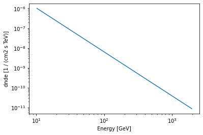
We assign the return axes object to variable called ax_crab_3fhl, because we will re-use it later to plot the flux points on top.
To compute the differential flux at 100 GeV we can simply call the model like normal Python function and convert to the desired units:
[29]:
crab_3fhl_spec(100 * u.GeV).to("cm-2 s-1 GeV-1")
[29]:
Next we can compute the integral flux of the Crab between 10 GeV and 2000 GeV:
[30]:
crab_3fhl_spec.integral(energy_min=10 * u.GeV, energy_max=2000 * u.GeV).to(
    "cm-2 s-1"
)
[30]:
We can easily convince ourself, that it corresponds to the value given in the Fermi-LAT 3FHL catalog:
[31]:
crab_3fhl.data["Flux"]
[31]:
In addition we can compute the energy flux between 10 GeV and 2000 GeV:
[32]:
crab_3fhl_spec.energy_flux(energy_min=10 * u.GeV, energy_max=2000 * u.GeV).to(
    "erg cm-2 s-1"
)
[32]:
Next we will access the flux points data of the Crab:
[33]:
print(crab_3fhl.flux_points)
FluxPoints
----------

  geom                   : RegionGeom
  axes                   : ['lon', 'lat', 'energy']
  shape                  : (1, 1, 5)
  quantities             : ['norm', 'norm_errp', 'norm_errn', 'norm_ul', 'sqrt_ts', 'is_ul']
  ref. model             : pl
  n_sigma                : 1
  n_sigma_ul             : 2
  sqrt_ts_threshold_ul   : 1
  sed type init          : flux
If you want to learn more about the different flux point formats you can read the specification here.
No we can check again the underlying astropy data structure by accessing the .table attribute:
[34]:
crab_3fhl.flux_points.to_table(sed_type="dnde", formatted=True)
[34]:
| e_ref | e_min | e_max | dnde | dnde_errp | dnde_errn | dnde_ul | sqrt_ts | is_ul |
|---|---|---|---|---|---|---|---|---|
| GeV | GeV | GeV | 1 / (cm2 GeV s) | 1 / (cm2 GeV s) | 1 / (cm2 GeV s) | 1 / (cm2 GeV s) | ||
| float64 | float64 | float64 | float64 | float64 | float64 | float64 | float32 | bool |
| 14.142 | 10.000 | 20.000 | 5.120e-10 | 1.321e-11 | 1.321e-11 | nan | 125.157 | False |
| 31.623 | 20.000 | 50.000 | 7.359e-11 | 2.842e-12 | 2.842e-12 | nan | 88.715 | False |
| 86.603 | 50.000 | 150.000 | 9.024e-12 | 5.367e-13 | 5.367e-13 | nan | 59.087 | False |
| 273.861 | 150.000 | 500.000 | 7.660e-13 | 8.707e-14 | 8.097e-14 | nan | 33.076 | False |
| 1000.000 | 500.000 | 2000.000 | 4.291e-14 | 1.086e-14 | 9.393e-15 | nan | 15.573 | False |
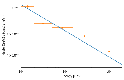
Finally let’s combine spectral model and flux points in a single plot and scale with energy_power=2 to obtain the spectral energy distribution:
[35]:
ax = crab_3fhl_spec.plot(energy_bounds=[10, 2000] * u.GeV, energy_power=2)
crab_3fhl.flux_points.plot(ax=ax, sed_type="dnde", energy_power=2);
Exercises
Plot the spectral model and flux points for PKS 2155-304 for the 3FGL and 2FHL catalogs. Try to plot the error of the model (aka “Butterfly”) as well. Note this requires the uncertainties package to be installed on your machine.
[ ]:
What next?
This was a quick introduction to some of the high level classes in Astropy and Gammapy.
To learn more about those classes, go to the API docs (links are in the introduction at the top).
To learn more about other parts of Gammapy (e.g. Fermi-LAT and TeV data analysis), check out the other tutorial notebooks.
To see what’s available in Gammapy, browse the Gammapy docs or use the full-text search.
If you have any questions, ask on the mailing list.