Naima spectral model

This class provides an interface with the models defined in the naima models module.

The model accepts as a positional argument a Naima radiative models instance, used to compute the non-thermal emission from populations of relativistic electrons or protons due to interactions with the ISM or with radiation and magnetic fields.

One of the advantages provided by this class consists in the possibility of performing a maximum likelihood spectral fit of the model’s parameters directly on observations, as opposed to the MCMC fit to flux points featured in Naima. All the parameters defining the parent population of charged particles are stored as Parameter and left free by default. In case that the radiative model is Synchrotron, the magnetic field strength may also be fitted. Parameters can be freezed/unfreezed before the fit, and maximum/minimum values can be set to limit the parameters space to the physically interesting region.

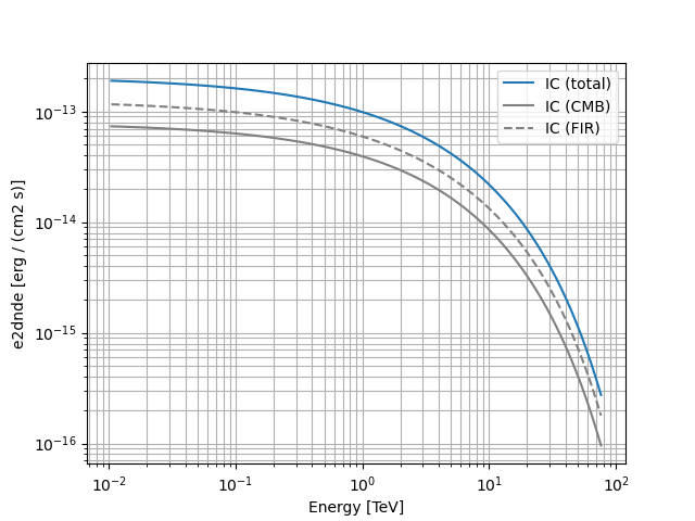
Example plot

Here we create and plot a spectral model that convolves an ExpCutoffPowerLawSpectralModel electron distribution with an InverseCompton radiative model, in the presence of multiple seed photon fields.

from astropy import units as u
import matplotlib.pyplot as plt
import naima
from gammapy.modeling.models import Models, NaimaSpectralModel, SkyModel

particle_distribution = naima.models.ExponentialCutoffPowerLaw(
    1e30 / u.eV, 10 * u.TeV, 3.0, 30 * u.TeV
)
radiative_model = naima.radiative.InverseCompton(
    particle_distribution,
    seed_photon_fields=["CMB", ["FIR", 26.5 * u.K, 0.415 * u.eV / u.cm ** 3]],
    Eemin=100 * u.GeV,
)

model = NaimaSpectralModel(radiative_model, distance=1.5 * u.kpc)

opts = {
    "energy_bounds": [10 * u.GeV, 80 * u.TeV],
    "sed_type": "e2dnde",
}

# Plot the total inverse Compton emission
model.plot(label="IC (total)", **opts)

# Plot the separate contributions from each seed photon field
for seed, ls in zip(["CMB", "FIR"], ["-", "--"]):
    model = NaimaSpectralModel(radiative_model, seed=seed, distance=1.5 * u.kpc)
    model.plot(label=f"IC ({seed})", ls=ls, color="gray", **opts)

plt.legend(loc="best")
plt.grid(which="both")

YAML representation

Here is an example YAML file using the model:

model = SkyModel(spectral_model=model, name="naima-model")
models = Models([model])

print(models.to_yaml())

Out:

components:
-   name: naima-model
    type: SkyModel
    spectral:
        type: NaimaSpectralModel
        parameters:
        -   name: amplitude
            value: 1.0e+30
            unit: eV-1
            error: 0
            min: .nan
            max: .nan
            frozen: false
            interp: lin
            scale_method: scale10
        -   name: e_0
            value: 10.0
            unit: TeV
            error: 0
            min: .nan
            max: .nan
            frozen: false
            interp: lin
            scale_method: scale10
        -   name: alpha
            value: 3.0
            unit: ''
            error: 0
            min: .nan
            max: .nan
            frozen: false
            interp: lin
            scale_method: scale10
        -   name: e_cutoff
            value: 30.0
            unit: TeV
            error: 0
            min: .nan
            max: .nan
            frozen: false
            interp: lin
            scale_method: scale10
        -   name: beta
            value: 1.0
            unit: ''
            error: 0
            min: .nan
            max: .nan
            frozen: false
            interp: lin
            scale_method: scale10