This is a fixed-text formatted version of a Jupyter notebook

Try online
You may download all the notebooks in the documentation as a tar file.
Source files: sed_fitting.ipynb | sed_fitting.py

Flux point fitting¶

Prerequisites¶

Some knowledge about retrieving information from catalogs, see the catalogs tutorial

Context¶

Some high level studies do not rely on reduced datasets with their IRFs but directly on higher level products such as flux points. This is not ideal because flux points already contain some hypothesis for the underlying spectral shape and the uncertainties they carry are usually simplified (e.g. symmetric gaussian errors). Yet, this is an efficient way to combine heterogeneous data.

Objective: fit spectral models to combined Fermi-LAT and IACT flux points.

Proposed approach¶

Here we will load, the spectral points from Fermi-LAT and TeV catalogs and fit them with various spectral models to find the best representation of the wide band spectrum.

The central class we’re going to use for this example analysis is:

gammapy.datasets.FluxPointsDataset

In addition we will work with the following data classes:

And the following spectral model classes:

Setup¶

Let us start with the usual IPython notebook and Python imports:

[1]:

%matplotlib inline
import matplotlib.pyplot as plt

[2]:

from astropy import units as u
from gammapy.modeling.models import (
    PowerLawSpectralModel,
    ExpCutoffPowerLawSpectralModel,
    LogParabolaSpectralModel,
    SkyModel,
)
from gammapy.estimators import FluxPoints
from gammapy.datasets import FluxPointsDataset, Datasets
from gammapy.catalog import CATALOG_REGISTRY
from gammapy.modeling import Fit

Load spectral points¶

For this analysis we choose to work with the source ‘HESS J1507-622’ and the associated Fermi-LAT sources ‘3FGL J1506.6-6219’ and ‘3FHL J1507.9-6228e’. We load the source catalogs, and then access source of interest by name:

[3]:

catalog_3fgl = CATALOG_REGISTRY.get_cls("3fgl")()
catalog_3fhl = CATALOG_REGISTRY.get_cls("3fhl")()
catalog_gammacat = CATALOG_REGISTRY.get_cls("gamma-cat")()

[4]:

source_fermi_3fgl = catalog_3fgl["3FGL J1506.6-6219"]
source_fermi_3fhl = catalog_3fhl["3FHL J1507.9-6228e"]
source_gammacat = catalog_gammacat["HESS J1507-622"]

The corresponding flux points data can be accessed with .flux_points attribute:

[5]:

dataset_gammacat = FluxPointsDataset(
    data=source_gammacat.flux_points, name="gammacat"
)
dataset_gammacat.data.to_table(sed_type="dnde", formatted=True)

[5]:

Table length=6

e_ref	e_min	e_max	dnde	dnde_errp	dnde_errn	is_ul
TeV	TeV	TeV	1 / (cm2 s TeV)	1 / (cm2 s TeV)	1 / (cm2 s TeV)
float64	float64	float64	float64	float64	float64	bool
0.861	0.639	1.159	2.291e-12	8.955e-13	8.705e-13	False
1.562	1.159	2.077	6.982e-13	2.304e-13	2.204e-13	False
2.764	2.077	3.677	1.691e-13	7.188e-14	6.759e-14	False
4.892	3.677	6.990	7.729e-14	2.607e-14	2.401e-14	False
9.989	6.990	16.435	1.033e-14	5.642e-15	5.063e-15	False
27.040	16.435	44.490	7.450e-16	7.260e-16	5.721e-16	False

[6]:

dataset_3fgl = FluxPointsDataset(
    data=source_fermi_3fgl.flux_points, name="3fgl"
)
dataset_3fgl.data.to_table(sed_type="dnde", formatted=True)

[6]:

Table length=5

e_ref	e_min	e_max	dnde	dnde_errp	dnde_errn	dnde_ul	sqrt_ts	is_ul
MeV	MeV	MeV	1 / (cm2 MeV s)	1 / (cm2 MeV s)	1 / (cm2 MeV s)	1 / (cm2 MeV s)
float64	float64	float64	float64	float64	float64	float64	float32	bool
173.205	100.000	300.000	1.798e-10	5.566e-11	5.710e-11	nan	2.843	False
547.723	300.000	1000.000	2.171e-13	1.689e-12	nan	3.595e-12	0.000	True
1732.051	1000.000	3000.000	2.528e-13	1.058e-13	9.991e-14	nan	2.661	False
5477.226	3000.000	10000.000	2.654e-14	8.936e-15	7.932e-15	nan	4.265	False
31622.777	10000.000	100000.000	1.274e-15	4.237e-16	3.658e-16	nan	5.774	False

[7]:

dataset_3fhl = FluxPointsDataset(
    data=source_fermi_3fhl.flux_points, name="3fhl"
)
dataset_3fhl.data.to_table(sed_type="dnde", formatted=True)

[7]:

Table length=5

e_ref	e_min	e_max	dnde	dnde_errp	dnde_errn	dnde_ul	sqrt_ts	is_ul
GeV	GeV	GeV	1 / (cm2 GeV s)	1 / (cm2 GeV s)	1 / (cm2 GeV s)	1 / (cm2 GeV s)
float64	float64	float64	float64	float64	float64	float64	float32	bool
14.142	10.000	20.000	9.288e-12	2.343e-12	2.128e-12	nan	5.660	False
31.623	20.000	50.000	2.777e-12	6.572e-13	5.818e-13	nan	6.940	False
86.603	50.000	150.000	2.335e-13	1.055e-13	8.554e-14	nan	3.835	False
273.861	150.000	500.000	6.411e-14	2.697e-14	2.133e-14	nan	5.697	False
1000.000	500.000	2000.000	9.188e-21	4.034e-15	nan	8.068e-15	0.000	True

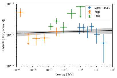
Power Law Fit¶

First we start with fitting a simple gammapy.modeling.models.PowerLawSpectralModel.

[8]:

pwl = PowerLawSpectralModel(
    index=2, amplitude="1e-12 cm-2 s-1 TeV-1", reference="1 TeV"
)
model = SkyModel(spectral_model=pwl, name="j1507-pl")

After creating the model we run the fit by passing the 'flux_points' and 'model' objects:

[9]:

datasets = Datasets([dataset_gammacat, dataset_3fgl, dataset_3fhl])
datasets.models = model
print(datasets)

Datasets
--------

Dataset 0:

  Type       : FluxPointsDataset
  Name       : gammacat
  Instrument :
  Models     : ['j1507-pl']

Dataset 1:

  Type       : FluxPointsDataset
  Name       : 3fgl
  Instrument :
  Models     : ['j1507-pl']

Dataset 2:

  Type       : FluxPointsDataset
  Name       : 3fhl
  Instrument :
  Models     : ['j1507-pl']

[10]:

fitter = Fit()
result_pwl = fitter.run(datasets=datasets)

And print the result:

[11]:

print(result_pwl)

OptimizeResult

        backend    : minuit
        method     : migrad
        success    : True
        message    : Optimization terminated successfully.
        nfev       : 40
        total stat : 28.29

OptimizeResult

        backend    : minuit
        method     : migrad
        success    : True
        message    : Optimization terminated successfully.
        nfev       : 40
        total stat : 28.29

[12]:

print(model)

SkyModel

  Name                      : j1507-pl
  Datasets names            : None
  Spectral model type       : PowerLawSpectralModel
  Spatial  model type       :
  Temporal model type       :
  Parameters:
    index                   :      1.985   +/-    0.03
    amplitude               :   1.28e-12   +/- 1.6e-13 1 / (cm2 s TeV)
    reference    (frozen)   :      1.000       TeV

Finally we plot the data points and the best fit model:

[13]:

ax = plt.subplot()

kwargs = {"ax": ax, "sed_type": "e2dnde", "yunits": u.Unit("TeV cm-2 s-1")}

for d in datasets:
    d.data.plot(label=d.name, **kwargs)

energy_bounds = [1e-4, 1e2] * u.TeV
pwl.plot(energy_bounds=energy_bounds, color="k", **kwargs)
pwl.plot_error(energy_bounds=energy_bounds, **kwargs)
ax.set_ylim(1e-13, 1e-11)
ax.set_xlim(energy_bounds)
ax.legend()

[13]:

<matplotlib.legend.Legend at 0x15a140a00>

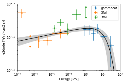
../../../_images/tutorials_analysis_1D_sed_fitting_21_1.png

Exponential Cut-Off Powerlaw Fit¶

Next we fit an gammapy.modeling.models.ExpCutoffPowerLawSpectralModel law to the data.

[14]:

ecpl = ExpCutoffPowerLawSpectralModel(
    index=1.8,
    amplitude="2e-12 cm-2 s-1 TeV-1",
    reference="1 TeV",
    lambda_="0.1 TeV-1",
)
model = SkyModel(spectral_model=ecpl, name="j1507-ecpl")

We run the fitter again by passing the flux points and the model instance:

[15]:

datasets.models = model
result_ecpl = fitter.run(datasets=datasets)
print(model)

SkyModel

  Name                      : j1507-ecpl
  Datasets names            : None
  Spectral model type       : ExpCutoffPowerLawSpectralModel
  Spatial  model type       :
  Temporal model type       :
  Parameters:
    index                   :      1.894   +/-    0.05
    amplitude               :   1.96e-12   +/- 3.9e-13 1 / (cm2 s TeV)
    reference    (frozen)   :      1.000       TeV
    lambda_                 :      0.078   +/-    0.05 1 / TeV
    alpha        (frozen)   :      1.000

We plot the data and best fit model:

[16]:

ax = plt.subplot()

kwargs = {"ax": ax, "sed_type": "e2dnde", "yunits": u.Unit("TeV cm-2 s-1")}

for d in datasets:
    d.data.plot(label=d.name, **kwargs)

ecpl.plot(energy_bounds=energy_bounds, color="k", **kwargs)
ecpl.plot_error(energy_bounds=energy_bounds, **kwargs)
ax.set_ylim(1e-13, 1e-11)
ax.set_xlim(energy_bounds)
ax.legend()

[16]:

<matplotlib.legend.Legend at 0x15a5ef640>

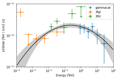
../../../_images/tutorials_analysis_1D_sed_fitting_27_1.png

Log-Parabola Fit¶

Finally we try to fit a gammapy.modeling.models.LogParabolaSpectralModel model:

[17]:

log_parabola = LogParabolaSpectralModel(
    alpha=2, amplitude="1e-12 cm-2 s-1 TeV-1", reference="1 TeV", beta=0.1
)
model = SkyModel(spectral_model=log_parabola, name="j1507-lp")

[18]:

datasets.models = model
result_log_parabola = fitter.run(datasets=datasets)
print(model)

SkyModel

  Name                      : j1507-lp
  Datasets names            : None
  Spectral model type       : LogParabolaSpectralModel
  Spatial  model type       :
  Temporal model type       :
  Parameters:
    amplitude               :   1.88e-12   +/- 2.8e-13 1 / (cm2 s TeV)
    reference    (frozen)   :      1.000       TeV
    alpha                   :      2.144   +/-    0.07
    beta                    :      0.049   +/-    0.02

[19]:

ax = plt.subplot()

kwargs = {"ax": ax, "sed_type": "e2dnde", "yunits": u.Unit("TeV cm-2 s-1")}

for d in datasets:
    d.data.plot(label=d.name, **kwargs)

log_parabola.plot(energy_bounds=energy_bounds, color="k", **kwargs)
log_parabola.plot_error(energy_bounds=energy_bounds, **kwargs)
ax.set_ylim(1e-13, 1e-11)
ax.set_xlim(energy_bounds)
ax.legend()

[19]:

<matplotlib.legend.Legend at 0x15ac05670>

../../../_images/tutorials_analysis_1D_sed_fitting_31_1.png

Exercises¶

Fit a gammapy.modeling.models.PowerLaw2SpectralModel and gammapy.modeling.models.ExpCutoffPowerLaw3FGLSpectralModel to the same data.
Fit a gammapy.modeling.models.ExpCutoffPowerLawSpectralModel model to Vela X (‘HESS J0835-455’) only and check if the best fit values correspond to the values given in the Gammacat catalog

What next?¶

This was an introduction to SED fitting in Gammapy.

If you would like to learn how to perform a full Poisson maximum likelihood spectral fit, please check out the spectrum analysis tutorial.
To learn how to combine heterogeneous datasets to perform a multi-instrument forward-folding fit see the MWL analysis tutorial

[ ]: