This is a fixed-text formatted version of a Jupyter notebook
Try online

You may download all the notebooks in the documentation as a tar file.
Source files: analysis_1.ipynb | analysis_1.py
High level interface
Prerequisites:
Understanding the gammapy data workflow, in particular what are DL3 events and instrument response functions (IRF).
Context
This notebook is an introduction to gammapy analysis using the high level interface.
Gammapy analysis consists in two main steps.
The first one is data reduction: user selected observations are reduced to a geometry defined by the user. It can be 1D (spectrum from a given extraction region) or 3D (with a sky projection and an energy axis). The resulting reduced data and instrument response functions (IRF) are called datasets in Gammapy.
The second step consists in setting a physical model on the datasets and fitting it to obtain relevant physical information.
Objective: Create a 3D dataset of the Crab using the H.E.S.S. DL3 data release 1 and perform a simple model fitting of the Crab nebula.
Proposed approach:
This notebook uses the high level Analysis class to orchestrate data reduction. In its current state, Analysis supports the standard analysis cases of joint or stacked 3D and 1D analyses. It is instantiated with an AnalysisConfig object that gives access to analysis parameters either directly or via a YAML config file.
To see what is happening under-the-hood and to get an idea of the internal API, a second notebook performs the same analysis without using the Analysis class.
In summary, we have to:
Create an
gammapy.analysis.AnalysisConfigobject and edit it to define the analysis configuration:Define what observations to use
Define the geometry of the dataset (data and IRFs)
Define the model we want to fit on the dataset.
Instantiate a
gammapy.analysis.Analysisfrom this configuration and run the different analysis stepsObservation selection
Data reduction
Model fitting
Estimating flux points
Finally we will compare the results against a reference model.
Setup
[1]:
%matplotlib inline
import matplotlib.pyplot as plt
[2]:
from pathlib import Path
from astropy import units as u
from gammapy.analysis import Analysis, AnalysisConfig
from gammapy.modeling.models import create_crab_spectral_model
Analysis configuration
For configuration of the analysis we use the YAML data format. YAML is a machine readable serialisation format, that is also friendly for humans to read. In this tutorial we will write the configuration file just using Python strings, but of course the file can be created and modified with any text editor of your choice.
Here is what the configuration for our analysis looks like:
[3]:
config = AnalysisConfig()
# the AnalysisConfig gives access to the various parameters used from logging to reduced dataset geometries
print(config)
AnalysisConfig

    general:
        log: {level: info, filename: null, filemode: null, format: null, datefmt: null}
        outdir: .
    observations:
        datastore: $GAMMAPY_DATA/hess-dl3-dr1
        obs_ids: []
        obs_file: null
        obs_cone: {frame: null, lon: null, lat: null, radius: null}
        obs_time: {start: null, stop: null}
        required_irf: [aeff, edisp, psf, bkg]
    datasets:
        type: 1d
        stack: true
        geom:
            wcs:
                skydir: {frame: null, lon: null, lat: null}
                binsize: 0.02 deg
                width: {width: 5.0 deg, height: 5.0 deg}
                binsize_irf: 0.2 deg
            selection: {offset_max: 2.5 deg}
            axes:
                energy: {min: 1.0 TeV, max: 10.0 TeV, nbins: 5}
                energy_true: {min: 0.5 TeV, max: 20.0 TeV, nbins: 16}
        map_selection: [counts, exposure, background, psf, edisp]
        background:
            method: null
            exclusion: null
            parameters: {}
        safe_mask:
            methods: [aeff-default]
            parameters: {}
        on_region: {frame: null, lon: null, lat: null, radius: null}
        containment_correction: true
    fit:
        fit_range: {min: null, max: null}
    flux_points:
        energy: {min: null, max: null, nbins: null}
        source: source
        parameters: {selection_optional: all}
    excess_map:
        correlation_radius: 0.1 deg
        parameters: {}
        energy_edges: {min: null, max: null, nbins: null}
    light_curve:
        time_intervals: {start: null, stop: null}
        energy_edges: {min: null, max: null, nbins: null}
        source: source
        parameters: {selection_optional: all}
Setting the data to use
We want to use Crab runs from the H.E.S.S. DL3-DR1. We define here the datastore and a cone search of observations pointing with 5 degrees of the Crab nebula. Parameters can be set directly or as a python dict.
PS: do not forget to setup your environment variable $GAMMAPY_DATA to your local directory containing the H.E.S.S. DL3-DR1 (see here).
[4]:
# We define the datastore containing the data
config.observations.datastore = "$GAMMAPY_DATA/hess-dl3-dr1"

# We define the cone search parameters
config.observations.obs_cone.frame = "icrs"
config.observations.obs_cone.lon = "83.633 deg"
config.observations.obs_cone.lat = "22.014 deg"
config.observations.obs_cone.radius = "5 deg"

# Equivalently we could have set parameters with a python dict
# config.observations.obs_cone = {"frame": "icrs", "lon": "83.633 deg", "lat": "22.014 deg", "radius": "5 deg"}
Setting the reduced datasets geometry
[5]:
# We want to perform a 3D analysis
config.datasets.type = "3d"
# We want to stack the data into a single reduced dataset
config.datasets.stack = True

# We fix the WCS geometry of the datasets
config.datasets.geom.wcs.skydir = {
    "lon": "83.633 deg",
    "lat": "22.014 deg",
    "frame": "icrs",
}
config.datasets.geom.wcs.width = {"width": "2 deg", "height": "2 deg"}
config.datasets.geom.wcs.binsize = "0.02 deg"

# We now fix the energy axis for the counts map
config.datasets.geom.axes.energy.min = "1 TeV"
config.datasets.geom.axes.energy.max = "10 TeV"
config.datasets.geom.axes.energy.nbins = 4

# We now fix the energy axis for the IRF maps (exposure, etc)
config.datasets.geom.axes.energy_true.min = "0.5 TeV"
config.datasets.geom.axes.energy_true.max = "20 TeV"
config.datasets.geom.axes.energy.nbins = 10
Setting the background normalization maker
[6]:
config.datasets.background.method = "fov_background"
config.datasets.background.parameters = {"method": "scale"}
Setting the exclusion mask
In order to properly adjust the background normalisation on regions without gamma-ray signal, one needs to define an exclusion mask for the background normalisation. For this tutorial, we use the following one $GAMMAPY_DATA/joint-crab/exclusion/exclusion_mask_crab.fits.gz
[7]:
config.datasets.background.exclusion = (
    "$GAMMAPY_DATA/joint-crab/exclusion/exclusion_mask_crab.fits.gz"
)
Setting modeling and fitting parameters
Analysis can perform a few modeling and fitting tasks besides data reduction. Parameters have then to be passed to the configuration object.
Here we define the energy range on which to perform the fit. We also set the energy edges used for flux point computation as well as the correlation radius to compute excess and significance maps.
[8]:
config.fit.fit_range.min = 1 * u.TeV
config.fit.fit_range.max = 10 * u.TeV
config.flux_points.energy = {"min": "1 TeV", "max": "10 TeV", "nbins": 3}
config.excess_map.correlation_radius = 0.1 * u.deg
We’re all set. But before we go on let’s see how to save or import AnalysisConfig objects though YAML files.
Using YAML configuration files
One can export/import the AnalysisConfig to/from a YAML file.
[9]:
config.write("config.yaml", overwrite=True)
[10]:
config = AnalysisConfig.read("config.yaml")
print(config)
AnalysisConfig

    general:
        log: {level: info, filename: null, filemode: null, format: null, datefmt: null}
        outdir: .
    observations:
        datastore: $GAMMAPY_DATA/hess-dl3-dr1
        obs_ids: []
        obs_file: null
        obs_cone: {frame: icrs, lon: 83.633 deg, lat: 22.014 deg, radius: 5.0 deg}
        obs_time: {start: null, stop: null}
        required_irf: [aeff, edisp, psf, bkg]
    datasets:
        type: 3d
        stack: true
        geom:
            wcs:
                skydir: {frame: icrs, lon: 83.633 deg, lat: 22.014 deg}
                binsize: 0.02 deg
                width: {width: 2.0 deg, height: 2.0 deg}
                binsize_irf: 0.2 deg
            selection: {offset_max: 2.5 deg}
            axes:
                energy: {min: 1.0 TeV, max: 10.0 TeV, nbins: 10}
                energy_true: {min: 0.5 TeV, max: 20.0 TeV, nbins: 16}
        map_selection: [counts, exposure, background, psf, edisp]
        background:
            method: fov_background
            exclusion: $GAMMAPY_DATA/joint-crab/exclusion/exclusion_mask_crab.fits.gz
            parameters: {method: scale}
        safe_mask:
            methods: [aeff-default]
            parameters: {}
        on_region: {frame: null, lon: null, lat: null, radius: null}
        containment_correction: true
    fit:
        fit_range: {min: 1.0 TeV, max: 10.0 TeV}
    flux_points:
        energy: {min: 1.0 TeV, max: 10.0 TeV, nbins: 3}
        source: source
        parameters: {selection_optional: all}
    excess_map:
        correlation_radius: 0.1 deg
        parameters: {}
        energy_edges: {min: null, max: null, nbins: null}
    light_curve:
        time_intervals: {start: null, stop: null}
        energy_edges: {min: null, max: null, nbins: null}
        source: source
        parameters: {selection_optional: all}
Running the analysis
We first create an gammapy.analysis.Analysis object from our configuration.
[11]:
analysis = Analysis(config)
Setting logging config: {'level': 'INFO', 'filename': None, 'filemode': None, 'format': None, 'datefmt': None}
Observation selection
We can directly select and load the observations from disk using gammapy.analysis.Analysis.get_observations():
[12]:
analysis.get_observations()
Fetching observations.
No HDU found matching: OBS_ID = 23523, HDU_TYPE = rad_max, HDU_CLASS = None
No HDU found matching: OBS_ID = 23526, HDU_TYPE = rad_max, HDU_CLASS = None
No HDU found matching: OBS_ID = 23559, HDU_TYPE = rad_max, HDU_CLASS = None
No HDU found matching: OBS_ID = 23592, HDU_TYPE = rad_max, HDU_CLASS = None
Number of selected observations: 4
The observations are now available on the Analysis object. The selection corresponds to the following ids:
[13]:
analysis.observations.ids
[13]:
['23523', '23526', '23559', '23592']
To see how to explore observations, please refer to the following notebook: CTA with Gammapy or HESS with Gammapy
Data reduction
Now we proceed to the data reduction. In the config file we have chosen a WCS map geometry, energy axis and decided to stack the maps. We can run the reduction using .get_datasets():
[14]:
%%time
analysis.get_datasets()
Creating reference dataset and makers.
Creating the background Maker.
Start the data reduction loop.
CPU times: user 1.75 s, sys: 88.9 ms, total: 1.84 s
Wall time: 1.84 s
As we have chosen to stack the data, there is finally one dataset contained which we can print:
[15]:
print(analysis.datasets["stacked"])
MapDataset
----------

  Name                            : stacked

  Total counts                    : 2485
  Total background counts         : 1997.49
  Total excess counts             : 487.51

  Predicted counts                : 1997.49
  Predicted background counts     : 1997.49
  Predicted excess counts         : nan

  Exposure min                    : 2.97e+08 m2 s
  Exposure max                    : 3.51e+09 m2 s

  Number of total bins            : 100000
  Number of fit bins              : 100000

  Fit statistic type              : cash
  Fit statistic value (-2 log(L)) : nan

  Number of models                : 0
  Number of parameters            : 0
  Number of free parameters       : 0
As you can see the dataset comes with a predefined background model out of the data reduction, but no source model has been set yet.
The counts, exposure and background model maps are directly available on the dataset and can be printed and plotted:
[16]:
counts = analysis.datasets["stacked"].counts
counts.smooth("0.05 deg").plot_interactive()
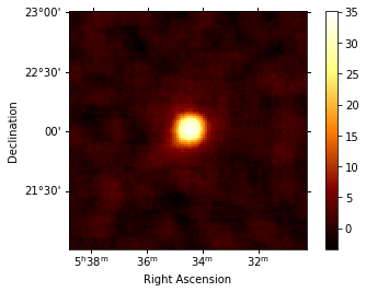
We can also compute the map of the sqrt_ts (significance) of the excess counts above the background. The correlation radius to sum counts is defined in the config file.
[17]:
analysis.get_excess_map()
analysis.excess_map["sqrt_ts"].plot(add_cbar=True);
Computing excess maps.
Save dataset to disk
It is common to run the preparation step independent of the likelihood fit, because often the preparation of maps, PSF and energy dispersion is slow if you have a lot of data. We first create a folder:
[18]:
path = Path("analysis_1")
path.mkdir(exist_ok=True)
And then write the maps and IRFs to disk by calling the dedicated write() method:
[19]:
filename = path / "crab-stacked-dataset.fits.gz"
analysis.datasets[0].write(filename, overwrite=True)
Model fitting
Now we define a model to be fitted to the dataset. Here we use its YAML definition to load it:
[20]:
model_config = """
components:
- name: crab
  type: SkyModel
  spatial:
    type: PointSpatialModel
    frame: icrs
    parameters:
    - name: lon_0
      value: 83.63
      unit: deg
    - name: lat_0
      value: 22.014
      unit: deg
  spectral:
    type: PowerLawSpectralModel
    parameters:
    - name: amplitude
      value: 1.0e-12
      unit: cm-2 s-1 TeV-1
    - name: index
      value: 2.0
      unit: ''
    - name: reference
      value: 1.0
      unit: TeV
      frozen: true
"""
Now we set the model on the analysis object:
[21]:
analysis.set_models(model_config)
Reading model.
Models

Component 0: SkyModel

  Name                      : crab
  Datasets names            : None
  Spectral model type       : PowerLawSpectralModel
  Spatial  model type       : PointSpatialModel
  Temporal model type       :
  Parameters:
    index                   :      2.000   +/-    0.00
    amplitude               :   1.00e-12   +/- 0.0e+00 1 / (cm2 s TeV)
    reference    (frozen)   :      1.000       TeV
    lon_0                   :     83.630   +/-    0.00 deg
    lat_0                   :     22.014   +/-    0.00 deg

Component 1: FoVBackgroundModel

  Name                      : stacked-bkg
  Datasets names            : ['stacked']
  Spectral model type       : PowerLawNormSpectralModel
  Parameters:
    norm                    :      1.000   +/-    0.00
    tilt         (frozen)   :      0.000
    reference    (frozen)   :      1.000       TeV
Finally we run the fit:
[22]:
analysis.run_fit()
Fitting datasets.
OptimizeResult

        backend    : minuit
        method     : migrad
        success    : True
        message    : Optimization terminated successfully.
        nfev       : 271
        total stat : 19992.17

OptimizeResult

        backend    : minuit
        method     : migrad
        success    : True
        message    : Optimization terminated successfully.
        nfev       : 271
        total stat : 19992.17
[23]:
print(analysis.fit_result)
OptimizeResult

        backend    : minuit
        method     : migrad
        success    : True
        message    : Optimization terminated successfully.
        nfev       : 271
        total stat : 19992.17

OptimizeResult

        backend    : minuit
        method     : migrad
        success    : True
        message    : Optimization terminated successfully.
        nfev       : 271
        total stat : 19992.17
This is how we can write the model back to file again:
[24]:
filename = path / "model-best-fit.yaml"
analysis.models.write(filename, overwrite=True)
[25]:
!cat analysis_1/model-best-fit.yaml
components:
-   name: crab
    type: SkyModel
    spectral:
        type: PowerLawSpectralModel
        parameters:
        -   name: index
            value: 2.5538019288289857
            error: 0.10302531554727902
        -   name: amplitude
            value: 4.529912786057623e-11
            unit: cm-2 s-1 TeV-1
            error: 3.7040387851201704e-12
        -   name: reference
            value: 1.0
            unit: TeV
            frozen: true
    spatial:
        type: PointSpatialModel
        frame: icrs
        parameters:
        -   name: lon_0
            value: 83.61981157931403
            unit: deg
            error: 0.003136890354033938
        -   name: lat_0
            value: 22.024556120192997
            unit: deg
            error: 0.002956430444973766
-   type: FoVBackgroundModel
    datasets_names:
    - stacked
    spectral:
        type: PowerLawNormSpectralModel
        parameters:
        -   name: norm
            value: 0.9864855339268036
            error: 0.023473292266494795
        -   name: tilt
            value: 0.0
            frozen: true
        -   name: reference
            value: 1.0
            unit: TeV
            frozen: true
covariance: model-best-fit_covariance.dat
Flux points
[26]:
analysis.config.flux_points.source = "crab"
analysis.get_flux_points()
Calculating flux points.
Reoptimize = False ignored for iminuit backend
Reoptimize = False ignored for iminuit backend
Reoptimize = False ignored for iminuit backend
Reoptimize = False ignored for iminuit backend
Reoptimize = False ignored for iminuit backend
Reoptimize = False ignored for iminuit backend

      e_ref                 dnde                 dnde_ul                dnde_err             sqrt_ts
       TeV            1 / (cm2 s TeV)        1 / (cm2 s TeV)        1 / (cm2 s TeV)
------------------ ---------------------- ---------------------- ---------------------- ------------------
1.4125375446227544 1.8458165524256397e-11 2.1070498239636086e-11 1.2545944678579331e-12  29.19604570871725
3.1622776601683795 2.4761998180771976e-12 2.9210092422785443e-12 2.1186999239487364e-13 24.242265531875965
 7.079457843841381 2.9304711864719196e-13 4.1958743058008545e-13  5.643875691976319e-14 11.764723730021181
[27]:
ax_sed, ax_residuals = analysis.flux_points.plot_fit()
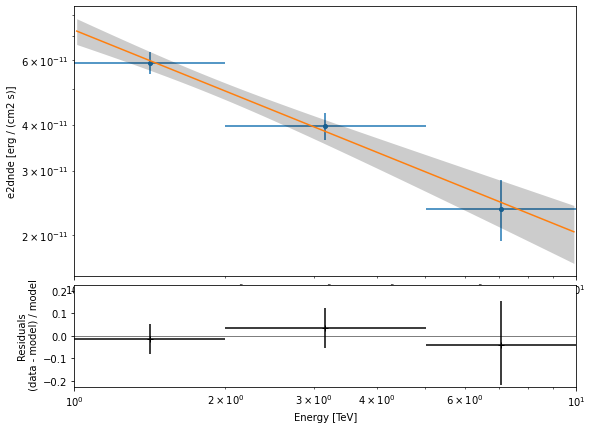
The flux points can be exported to a fits table following the format defined here
[28]:
filename = path / "flux-points.fits"
analysis.flux_points.write(filename, overwrite=True)
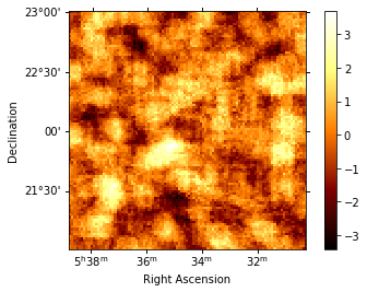
To check the fit is correct, we compute the map of the sqrt_ts of the excess counts above the current model.
[29]:
analysis.get_excess_map()
analysis.excess_map["sqrt_ts"].plot(add_cbar=True);
Computing excess maps.
What’s next
You can look at the same analysis without the high level interface in analysis_2
You can see how to perform a 1D spectral analysis of the same data in spectrum analysis
[ ]: