This is a fixed-text formatted version of a Jupyter notebook
Try online

You may download all the notebooks in the documentation as a tar file.
Source files: catalog.ipynb | catalog.py
Source catalogs
gammapy.catalog provides convenient access to common gamma-ray source catalogs. This module is mostly independent from the rest of Gammapy. Typically you use it to compare new analyses against catalog results, e.g. overplot the spectral model, or compare the source position.
Moreover as creating a source model and flux points for a given catalog from the FITS table is tedious, gammapy.catalog has this already implemented. So you can create initial source models for your analyses. This is very common for Fermi-LAT, to start with a catalog model. For TeV analysis, especially in crowded Galactic regions, using the HGPS, gamma-cat or 2HWC catalog in this way can also be useful.
In this tutorial you will learn how to:
List available catalogs
Load a catalog
Access the source catalog table data
Select a catalog subset or a single source
Get source spectral and spatial models
Get flux points (if available)
Get lightcurves (if available)
Access the source catalog table data
Pretty-print the source information
In this tutorial we will show examples using the following catalogs:
All catalog and source classes work the same, as long as some information is available. E.g. trying to access a lightcurve from a catalog and source that doesn’t have that information will return None.
Further information is available at gammapy.catalog.
[1]:
%matplotlib inline
import numpy as np
import matplotlib.pyplot as plt
import astropy.units as u
from gammapy.catalog import CATALOG_REGISTRY
List available catalogs
gammapy.catalog contains a catalog registry CATALOG_REGISTRY, which maps catalog names (e.g. “3fhl”) to catalog classes (e.g. SourceCatalog3FHL).
[2]:
CATALOG_REGISTRY
[2]:
[gammapy.catalog.gammacat.SourceCatalogGammaCat,
 gammapy.catalog.hess.SourceCatalogHGPS,
 gammapy.catalog.hawc.SourceCatalog2HWC,
 gammapy.catalog.fermi.SourceCatalog3FGL,
 gammapy.catalog.fermi.SourceCatalog4FGL,
 gammapy.catalog.fermi.SourceCatalog2FHL,
 gammapy.catalog.fermi.SourceCatalog3FHL,
 gammapy.catalog.hawc.SourceCatalog3HWC]
Load catalogs
If you have run gammapy download datasets or gammapy download tutorials, you have a copy of the catalogs as FITS files in $GAMMAPY_DATA/catalogs, and that is the default location where gammapy.catalog loads from.
[3]:
!ls -1 $GAMMAPY_DATA/catalogs
2HWC.ecsv
2HWC.yaml
3HWC.ecsv
3HWC.yaml
README.rst
fermi
gammacat
hgps_catalog_v1.fits.gz
make_2hwc.py
make_3hwc.py
[4]:
!ls -1 $GAMMAPY_DATA/catalogs/fermi
Extended_archive_v15
Extended_archive_v18
LAT_extended_sources_8years
README.rst
gll_psc_v16.fit.gz
gll_psc_v20.fit.gz
gll_psc_v27.fit.gz
gll_psch_v08.fit.gz
gll_psch_v09.fit.gz
gll_psch_v13.fit.gz
So a catalog can be loaded directly from its corresponding class
[5]:
from gammapy.catalog import SourceCatalog4FGL

catalog = SourceCatalog4FGL()
print("Number of sources :", len(catalog.table))
Number of sources : 5788
Note that it loads the default catalog from $GAMMAPY_DATA/catalogs, you could pass a different filename when creating the catalog. For example here we load an older version of 4FGL catalog:
[6]:
catalog = SourceCatalog4FGL("$GAMMAPY_DATA/catalogs/fermi/gll_psc_v20.fit.gz")
print("Number of sources :", len(catalog.table))
Number of sources : 5066
Alternatively you can load a catalog by name via CATALOG_REGISTRY.get_cls(name)() (note the () to instantiate a catalog object from the catalog class - only this will load the catalog and be useful), or by importing the catalog class (e.g. SourceCatalog3FGL) directly. The two ways are equivalent, the result will be the same.
[7]:
# FITS file is loaded
catalog = CATALOG_REGISTRY.get_cls("3fgl")()
catalog
[7]:
<gammapy.catalog.fermi.SourceCatalog3FGL at 0x1283dc070>
[8]:
# Let's load the source catalogs we will use throughout this tutorial
catalog_gammacat = CATALOG_REGISTRY.get_cls("gamma-cat")()
catalog_3fhl = CATALOG_REGISTRY.get_cls("3fhl")()
catalog_4fgl = CATALOG_REGISTRY.get_cls("4fgl")()
catalog_hgps = CATALOG_REGISTRY.get_cls("hgps")()
Catalog table
Source catalogs are given as FITS files that contain one or multiple tables.
However, you can also access the underlying astropy.table.Table for a catalog, and the row data as a Python dict. This can be useful if you want to do something that is not pre-scripted by the gammapy.catalog classes, such as e.g. selecting sources by sky position or association class, or accessing special source information.
[9]:
type(catalog_3fhl.table)
[9]:
astropy.table.table.Table
[10]:
len(catalog_3fhl.table)
[10]:
1556
[11]:
catalog_3fhl.table[:3][["Source_Name", "RAJ2000", "DEJ2000"]]
[11]:
| Source_Name | RAJ2000 | DEJ2000 |
|---|---|---|
| deg | deg | |
| bytes18 | float32 | float32 |
| 3FHL J0001.2-0748 | 0.3107 | -7.8075 |
| 3FHL J0001.9-4155 | 0.4849 | -41.9303 |
| 3FHL J0002.1-6728 | 0.5283 | -67.4825 |
Note that the catalogs object include a helper property that gives directly the sources positions as a SkyCoord object (we will show an usage example in the following).
[12]:
catalog_3fhl.positions[:3]
[12]:
<SkyCoord (ICRS): (ra, dec) in deg
    [(0.31067517,  -7.8075185), (0.4848653 , -41.93026  ),
     (0.52826166, -67.48248  )]>
Source object
Select a source
The catalog entries for a single source are represented by a SourceCatalogObject. In order to select a source object index into the catalog using [], with a catalog table row index (zero-based, first row is [0]), or a source name. If a name is given, catalog table columns with source names and association names (“ASSOC1” in the example below) are searched top to bottom. There is no name resolution web query.
[13]:
source = catalog_4fgl[49]
source
[13]:
<gammapy.catalog.fermi.SourceCatalogObject4FGL at 0x1283e46a0>
[14]:
source.row_index, source.name
[14]:
(49, '4FGL J0010.8-2154')
[15]:
source = catalog_4fgl["4FGL J0010.8-2154"]
source.row_index, source.name
[15]:
(49, '4FGL J0010.8-2154')
[16]:
source.data["ASSOC1"]
[16]:
'PKS 0008-222 '
[17]:
source = catalog_4fgl["PKS 0008-222"]
source.row_index, source.name
[17]:
(49, '4FGL J0010.8-2154')
Note that you can also do a for source in catalog loop, to find or process sources of interest.
Source information
The source objects have a data property that contains the information of the catalog row corresponding to the source.
[18]:
source.data["Npred"]
[18]:
276.04663
[19]:
source.data["GLON"], source.data["GLAT"]
[19]:
(<Quantity 60.28118 deg>, <Quantity -79.400505 deg>)
As for the catalog object, the source object has a position property.
[20]:
source.position.galactic
[20]:
<SkyCoord (Galactic): (l, b) in deg
    (60.28120079, -79.40051035)>
Select a catalog subset
The catalog objects support selection using boolean arrays (of the same length), so one can create a new catalog as a subset of the main catalog that verify a set of conditions.
In the next example we selection only few of the brightest sources brightest sources in the 100 to 200 GeV energy band.
[21]:
mask_bright = np.zeros(len(catalog_3fhl.table), dtype=bool)
for k, source in enumerate(catalog_3fhl):
    flux = (
        source.spectral_model()
        .integral(100 * u.GeV, 200 * u.GeV)
        .to("cm-2 s-1")
    )
    if flux > 1e-10 * u.Unit("cm-2 s-1"):
        mask_bright[k] = True
        print(f"{source.row_index:<7d} {source.name:20s} {flux:.3g}")
352     3FHL J0534.5+2201    2.99e-10 1 / (cm2 s)
553     3FHL J0851.9-4620e   1.24e-10 1 / (cm2 s)
654     3FHL J1036.3-5833e   1.57e-10 1 / (cm2 s)
691     3FHL J1104.4+3812    3.34e-10 1 / (cm2 s)
1111    3FHL J1653.8+3945    1.27e-10 1 / (cm2 s)
1219    3FHL J1824.5-1351e   1.77e-10 1 / (cm2 s)
1361    3FHL J2028.6+4110e   1.75e-10 1 / (cm2 s)
[22]:
catalog_3fhl_bright = catalog_3fhl[mask_bright]
catalog_3fhl_bright
[22]:
<gammapy.catalog.fermi.SourceCatalog3FHL at 0x1283ee460>
[23]:
catalog_3fhl_bright.table["Source_Name"]
[23]:
| 3FHL J0534.5+2201 |
| 3FHL J0851.9-4620e |
| 3FHL J1036.3-5833e |
| 3FHL J1104.4+3812 |
| 3FHL J1653.8+3945 |
| 3FHL J1824.5-1351e |
| 3FHL J2028.6+4110e |
Similarly we can select only sources within a region of interest. Here for example we use the position property of the catalog object to select sources whitin 5 degrees from “PKS 0008-222”:
[24]:
source = catalog_4fgl["PKS 0008-222"]
mask_roi = source.position.separation(catalog_4fgl.positions) < 5 * u.deg
[25]:
catalog_4fgl_roi = catalog_4fgl[mask_roi]
print("Number of sources :", len(catalog_4fgl_roi.table))
Number of sources : 11
Source models
The gammapy.catalog.SourceCatalogObject classes have a sky_model() model which creates a gammapy.modeling.models.SkyModel object, with model parameter values and parameter errors from the catalog filled in.
In most cases, the spectral_model() method provides the gammapy.modeling.models.SpectralModel part of the sky model, and the spatial_model() method the gammapy.modeling.models.SpatialModel part individually.
We use the gammapy.catalog.SourceCatalog3FHL for the examples in this section.
[26]:
source = catalog_4fgl["PKS 2155-304"]
[27]:
model = source.sky_model()
model
[27]:
SkyModel(spatial_model=<gammapy.modeling.models.spatial.PointSpatialModel object at 0x128724430>, spectral_model=<gammapy.modeling.models.spectral.LogParabolaSpectralModel object at 0x128724940>)temporal_model=None)
[28]:
print(model)
SkyModel

  Name                      : 4FGL J2158.8-3013
  Datasets names            : None
  Spectral model type       : LogParabolaSpectralModel
  Spatial  model type       : PointSpatialModel
  Temporal model type       :
  Parameters:
    amplitude               :   1.44e-11   +/- 1.7e-13 1 / (cm2 MeV s)
    reference    (frozen)   :   1118.643       MeV
    alpha                   :      1.767   +/-    0.01
    beta                    :      0.041   +/-    0.00
    lon_0                   :    329.714   +/-    0.00 deg
    lat_0                   :    -30.225   +/-    0.00 deg
[29]:
print(model.spatial_model)
PointSpatialModel

  type   name    value    unit   error      min        max    frozen link
------- ----- ----------- ---- --------- ---------- --------- ------ ----
spatial lon_0  3.2971e+02  deg 3.735e-03        nan       nan  False
spatial lat_0 -3.0225e+01  deg 3.227e-03 -9.000e+01 9.000e+01  False
[30]:
print(model.spectral_model)
LogParabolaSpectralModel

  type      name     value         unit        error   min max frozen link
-------- --------- ---------- -------------- --------- --- --- ------ ----
spectral amplitude 1.4365e-11 cm-2 MeV-1 s-1 1.655e-13 nan nan  False
spectral reference 1.1186e+03            MeV 0.000e+00 nan nan   True
spectral     alpha 1.7668e+00                1.163e-02 nan nan  False
spectral      beta 4.0969e-02                4.120e-03 nan nan  False
[31]:
energy_bounds = (100 * u.MeV, 100 * u.GeV)
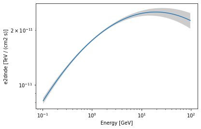
opts = dict(sed_type="e2dnde", yunits=u.Unit("TeV cm-2 s-1"))
model.spectral_model.plot(energy_bounds, **opts)
model.spectral_model.plot_error(energy_bounds, **opts);
You can create initial source models for your analyses using the .to_models() method of the catalog objects. Here for example we create a Models object from the 4FGL catalog subset we previously defined:
[32]:
models_4fgl_roi = catalog_4fgl_roi.to_models()
models_4fgl_roi
[32]:
<gammapy.modeling.models.core.Models at 0x12872b940>
Specificities of the HGPS catalog
Using the .to_models() method for the gammapy.catalog.SourceCatalogHGPS will return only the models components of the sources retained in the main catalog, several candidate objects appears only in the Gaussian components table (see section 4.9 of the HGPS paper, https://arxiv.org/abs/1804.02432). To access these components you can do the following:
[33]:
discarded_ind = np.where(
    [
        "Discarded" in _
        for _ in catalog_hgps.table_components["Component_Class"]
    ]
)[0]
discarded_table = catalog_hgps.table_components[discarded_ind]
There is no spectral model available for these components but you can access their spatial models:
[34]:
discarded_spatial = [
    catalog_hgps.gaussian_component(idx).spatial_model()
    for idx in discarded_ind
]
In addition to the source components the HGPS catalog include a large scale diffuse component built by fitting a gaussian model in a sliding window along the Galactic plane. Information on this model can be accessed via the propoerties .table_large_scale_component and .large_scale_component of gammapy.catalog.SourceCatalogHGPS.
[35]:
# here we show the 5 first elements of the table
catalog_hgps.table_large_scale_component[:5]
# you can also try :
# help(catalog_hgps.large_scale_component)
[35]:
| GLON | GLAT | GLAT_Err | Surface_Brightness | Surface_Brightness_Err | Width | Width_Err |
|---|---|---|---|---|---|---|
| deg | deg | deg | 1 / (cm2 s sr) | 1 / (cm2 s sr) | deg | deg |
| float32 | float32 | float32 | float32 | float32 | float32 | float32 |
| 270.000000 | 0.205357 | 0.251932 | 6.149827e-10 | 4.064108e-10 | 0.269385 | 0.137990 |
| 272.959198 | -0.120154 | 0.058201 | 1.426735e-09 | 7.346488e-10 | 0.088742 | 0.041882 |
| 275.918365 | -0.095232 | 0.089881 | 1.193710e-09 | 6.117877e-10 | 0.167219 | 0.111797 |
| 278.877563 | -0.257642 | 0.065071 | 1.506986e-09 | 5.230542e-10 | 0.156525 | 0.056130 |
| 281.836731 | -0.283487 | 0.066442 | 1.636973e-09 | 4.336444e-10 | 0.205192 | 0.049676 |
Flux points
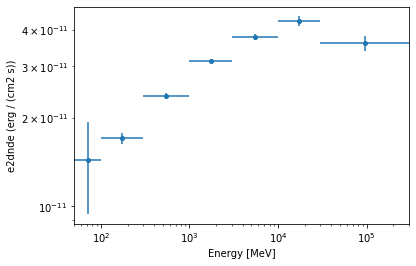
The flux points are available via the flux_points property as a gammapy.spectrum.FluxPoints object.
[36]:
source = catalog_4fgl["PKS 2155-304"]
flux_points = source.flux_points
[37]:
flux_points
[37]:
<gammapy.estimators.points.core.FluxPoints at 0x128af9d00>
[38]:
flux_points.to_table(sed_type="flux")
[38]:
| e_ref | e_min | e_max | flux | flux_errp | flux_errn | flux_ul | sqrt_ts | is_ul |
|---|---|---|---|---|---|---|---|---|
| MeV | MeV | MeV | 1 / (cm2 s) | 1 / (cm2 s) | 1 / (cm2 s) | 1 / (cm2 s) | ||
| float64 | float64 | float64 | float64 | float64 | float64 | float64 | float32 | bool |
| 70.71067811865478 | 49.99999999999999 | 100.00000000000004 | 8.811208118686409e-08 | 3.097255785178277e-08 | 3.039940565940924e-08 | nan | 2.5337915 | False |
| 173.20508075688775 | 100.00000000000004 | 299.99999999999994 | 6.859372092549165e-08 | 3.0207172319052233e-09 | 3.0207172319052233e-09 | nan | 25.057798 | False |
| 547.722557505166 | 299.99999999999994 | 999.9999999999998 | 3.348723609519766e-08 | 6.225928661507396e-10 | 6.225928661507396e-10 | nan | 88.745026 | False |
| 1732.0508075688763 | 999.9999999999998 | 2999.9999999999977 | 1.274911376469845e-08 | 2.198041054723987e-10 | 2.198041054723987e-10 | nan | 128.2931 | False |
| 5477.225575051666 | 2999.9999999999977 | 10000.00000000001 | 5.410327741373067e-09 | 1.2490801448716837e-10 | 1.2490801448716837e-10 | nan | 120.772316 | False |
| 17320.50807568877 | 10000.00000000001 | 30000.000000000007 | 1.7687512565700558e-09 | 6.802798602212334e-11 | 6.802798602212334e-11 | nan | 82.056656 | False |
| 94868.32980505146 | 30000.000000000007 | 299999.9999999999 | 6.965684695714458e-10 | 4.1411239021238444e-11 | 4.1411239021238444e-11 | nan | 54.02705 | False |
[39]:
flux_points.plot(sed_type="e2dnde");
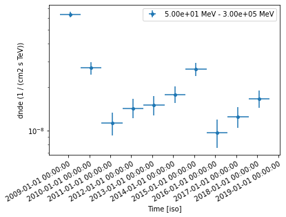
Lightcurves
The Fermi catalogs contain lightcurves for each source. It is available via the source.lightcurve() method as a gammapy.estimators.LightCurve object.
[40]:
lightcurve = catalog_4fgl["4FGL J0349.8-2103"].lightcurve()
[41]:
lightcurve
[41]:
<gammapy.estimators.points.core.FluxPoints at 0x128ec3910>
[42]:
lightcurve.to_table(format="lightcurve", sed_type="flux")
[42]:
| time_min | time_max | e_ref [1] | e_min [1] | e_max [1] | flux [1] | flux_errp [1] | flux_errn [1] | flux_ul [1] | ts [1] | sqrt_ts [1] | is_ul [1] |
|---|---|---|---|---|---|---|---|---|---|---|---|
| MeV | MeV | MeV | 1 / (cm2 s) | 1 / (cm2 s) | 1 / (cm2 s) | 1 / (cm2 s) | |||||
| float64 | float64 | float64 | float64 | float64 | float64 | float64 | float64 | float64 | float32 | float32 | bool |
| 54682.65603794185 | 55045.301668796295 | 3872.9833462074166 | 49.99999999999999 | 299999.9999999999 | 8.182966837466665e-08 | 4.0442960091979785e-09 | 4.0442960091979785e-09 | 8.991825950488419e-08 | 866.5454 | 29.437143 | False |
| 55045.301668796295 | 55410.57944657407 | 3872.9833462074166 | 49.99999999999999 | 299999.9999999999 | 3.4780882174345606e-08 | 3.377941926174799e-09 | 3.377941926174799e-09 | 4.1536765138516785e-08 | 177.31786 | 13.316075 | False |
| 55410.57944657407 | 55775.85722435185 | 3872.9833462074166 | 49.99999999999999 | 299999.9999999999 | 1.4417943283717705e-08 | 2.6934492414198985e-09 | 2.530577081216734e-09 | 1.980484221064671e-08 | 45.33303 | 6.7329807 | False |
| 55775.85722435185 | 56141.13500212963 | 3872.9833462074166 | 49.99999999999999 | 299999.9999999999 | 1.8312720229118895e-08 | 2.9073525809053535e-09 | 2.697997159017973e-09 | 2.4127425390929602e-08 | 69.82312 | 8.356023 | False |
| 56141.13500212963 | 56506.412779907405 | 3872.9833462074166 | 49.99999999999999 | 299999.9999999999 | 1.929730331085011e-08 | 3.0470421741313203e-09 | 2.900109263848094e-09 | 2.5391386770934332e-08 | 63.285576 | 7.955223 | False |
| 56506.412779907405 | 56871.690557685186 | 3872.9833462074166 | 49.99999999999999 | 299999.9999999999 | 2.279863409171412e-08 | 3.0816984519788093e-09 | 2.9492861486346555e-09 | 2.896203099567174e-08 | 98.43889 | 9.921638 | False |
| 56871.690557685186 | 57236.96833546296 | 3872.9833462074166 | 49.99999999999999 | 299999.9999999999 | 3.4101141466180707e-08 | 3.5666940512157908e-09 | 3.438366702468443e-09 | 4.123452868043387e-08 | 164.55066 | 12.82773 | False |
| 57236.96833546296 | 57602.24611324074 | 3872.9833462074166 | 49.99999999999999 | 299999.9999999999 | 1.2460412257553344e-08 | 2.889906092207184e-09 | 2.7565447702215806e-09 | 1.824022533014613e-08 | 26.10482 | 5.1092877 | False |
| 57602.24611324074 | 57967.523891018514 | 3872.9833462074166 | 49.99999999999999 | 299999.9999999999 | 1.5963367516746985e-08 | 2.667339016326764e-09 | 2.5512609802547104e-09 | 2.1298045993489723e-08 | 57.259422 | 7.5669956 | False |
| 57967.523891018514 | 58332.801668796295 | 3872.9833462074166 | 49.99999999999999 | 299999.9999999999 | 2.1374123804207557e-08 | 2.9909645871128987e-09 | 2.8739282065259886e-09 | 2.7356053422522567e-08 | 84.4538 | 9.189875 | False |
[43]:
lightcurve.plot();
Pretty-print source information
A source object has a nice string representation that you can print.
[44]:
source = catalog_hgps["MSH 15-52"]
print(source)
*** Basic info ***

Catalog row index (zero-based) : 18
Source name          : HESS J1514-591
Analysis reference   : HGPS
Source class         : PWN
Identified object    : MSH 15-52
Gamma-Cat id         : 79


*** Info from map analysis ***

RA                   :  228.499 deg = 15h14m00s
DEC                  :  -59.161 deg = -59d09m41s
GLON                 :  320.315 +/- 0.008 deg
GLAT                 :   -1.188 +/- 0.007 deg
Position Error (68%) : 0.020 deg
Position Error (95%) : 0.033 deg
ROI number           : 13
Spatial model        : 3-Gaussian
Spatial components   : HGPSC 023, HGPSC 024, HGPSC 025
TS                   : 1763.4
sqrt(TS)             : 42.0
Size                 : 0.145 +/- 0.026 (UL: 0.000) deg
R70                  : 0.215 deg
RSpec                : 0.215 deg
Total model excess   : 3502.8
Excess in RSpec      : 2440.5
Model Excess in RSpec : 2414.3
Background in RSpec  : 1052.5
Livetime             : 41.4 hours
Energy threshold     : 0.61 TeV
Source flux (>1 TeV) : (6.434 +/- 0.211) x 10^-12 cm^-2 s^-1 = (28.47 +/- 0.94) % Crab

Fluxes in RSpec (> 1 TeV):
Map measurement                : 4.552 x 10^-12 cm^-2 s^-1 = 20.14 % Crab
Source model                   : 4.505 x 10^-12 cm^-2 s^-1 = 19.94 % Crab
Other component model          : 0.000 x 10^-12 cm^-2 s^-1 =  0.00 % Crab
Large scale component model    : 0.000 x 10^-12 cm^-2 s^-1 =  0.00 % Crab
Total model                    : 4.505 x 10^-12 cm^-2 s^-1 = 19.94 % Crab
Containment in RSpec                :  70.0 %
Contamination in RSpec              :   0.0 %
Flux correction (RSpec -> Total)    : 142.8 %
Flux correction (Total -> RSpec)    :  70.0 %

*** Info from spectral analysis ***

Livetime             : 13.7 hours
Energy range:        : 0.38 to 61.90 TeV
Background           : 1825.9
Excess               : 2061.1
Spectral model       : ECPL
TS ECPL over PL      : 10.2
Best-fit model flux(> 1 TeV) : (5.720 +/- 0.417) x 10^-12 cm^-2 s^-1  = (25.31 +/- 1.84) % Crab
Best-fit model energy flux(1 to 10 TeV) : (20.779 +/- 1.878) x 10^-12 erg cm^-2 s^-1
Pivot energy         : 1.54 TeV
Flux at pivot energy : (2.579 +/- 0.083) x 10^-12 cm^-2 s^-1 TeV^-1  = (11.41 +/- 0.24) % Crab
PL   Flux(> 1 TeV)   : (5.437 +/- 0.186) x 10^-12 cm^-2 s^-1  = (24.06 +/- 0.82) % Crab
PL   Flux(@ 1 TeV)   : (6.868 +/- 0.241) x 10^-12 cm^-2 s^-1 TeV^-1  = (30.39 +/- 0.69) % Crab
PL   Index           : 2.26 +/- 0.03
ECPL   Flux(@ 1 TeV) : (6.860 +/- 0.252) x 10^-12 cm^-2 s^-1 TeV^-1  = (30.35 +/- 0.72) % Crab
ECPL   Flux(> 1 TeV) : (5.720 +/- 0.417) x 10^-12 cm^-2 s^-1  = (25.31 +/- 1.84) % Crab
ECPL Index           : 2.05 +/- 0.06
ECPL Lambda          : 0.052 +/- 0.014 TeV^-1
ECPL E_cut           : 19.20 +/- 5.01 TeV

*** Flux points info ***

Number of flux points: 6
Flux points table:

e_ref  e_min  e_max        dnde         dnde_errn       dnde_errp        dnde_ul     is_ul
 TeV    TeV    TeV   1 / (cm2 s TeV) 1 / (cm2 s TeV) 1 / (cm2 s TeV) 1 / (cm2 s TeV)
------ ------ ------ --------------- --------------- --------------- --------------- -----
 0.562  0.383  0.825       2.439e-11       1.419e-12       1.509e-12       2.732e-11 False
 1.212  0.825  1.778       4.439e-12       2.489e-13       2.654e-13       4.970e-12 False
 2.738  1.778  4.217       7.295e-13       4.788e-14       4.898e-14       8.302e-13 False
 6.190  4.217  9.085       1.305e-13       1.220e-14       1.282e-14       1.571e-13 False
13.991  9.085 21.544       1.994e-14       2.723e-15       2.858e-15       2.588e-14 False
31.623 21.544 46.416       9.474e-16       3.480e-16       4.329e-16       1.919e-15 False

*** Gaussian component info ***

Number of components: 3
Spatial components   : HGPSC 023, HGPSC 024, HGPSC 025

Component HGPSC 023:
GLON                 :  320.303 +/- 0.005 deg
GLAT                 :   -1.124 +/- 0.007 deg
Size                 : 0.057 +/- 0.005 deg
Flux (>1 TeV)        : (2.01 +/- 0.23) x 10^-12 cm^-2 s^-1 = (8.9 +/- 1.0) % Crab

Component HGPSC 024:
GLON                 :  320.298 +/- 0.020 deg
GLAT                 :   -1.168 +/- 0.021 deg
Size                 : 0.206 +/- 0.020 deg
Flux (>1 TeV)        : (2.54 +/- 0.29) x 10^-12 cm^-2 s^-1 = (11.2 +/- 1.3) % Crab

Component HGPSC 025:
GLON                 :  320.351 +/- 0.005 deg
GLAT                 :   -1.284 +/- 0.007 deg
Size                 : 0.055 +/- 0.005 deg
Flux (>1 TeV)        : (1.88 +/- 0.22) x 10^-12 cm^-2 s^-1 = (8.3 +/- 1.0) % Crab


*** Source associations info ***

  Source_Name    Association_Catalog    Association_Name   Separation
                                                              deg
---------------- ------------------- --------------------- ----------
  HESS J1514-591                2FHL    2FHL J1514.0-5915e   0.098903
  HESS J1514-591                3FGL     3FGL J1513.9-5908   0.026914
  HESS J1514-591                3FGL    3FGL J1514.0-5915e   0.094834
  HESS J1514-591                COMP            G320.4-1.2   0.070483
  HESS J1514-591                 PSR              B1509-58   0.026891

*** Source identification info ***

Source_Name: HESS J1514-591
Identified_Object: MSH 15-52
Class: PWN
Evidence: Morphology
Reference: 2005A%26A...435L..17A
Distance_Reference: SNRCat
Distance: 5.199999809265137 kpc
Distance_Min: 3.799999952316284 kpc
Distance_Max: 6.599999904632568 kpc
You can also call source.info() instead and pass as an option what information to print. The options available depend on the catalog, you can learn about them using help()
[45]:
help(source.info)
Help on method info in module gammapy.catalog.hess:

info(info='all') method of gammapy.catalog.hess.SourceCatalogObjectHGPS instance
    Info string.

    Parameters
    ----------
    info : {'all', 'basic', 'map', 'spec', 'flux_points', 'components', 'associations', 'id'}
        Comma separated list of options
[46]:
print(source.info("associations"))
*** Source associations info ***

  Source_Name    Association_Catalog    Association_Name   Separation
                                                              deg
---------------- ------------------- --------------------- ----------
  HESS J1514-591                2FHL    2FHL J1514.0-5915e   0.098903
  HESS J1514-591                3FGL     3FGL J1513.9-5908   0.026914
  HESS J1514-591                3FGL    3FGL J1514.0-5915e   0.094834
  HESS J1514-591                COMP            G320.4-1.2   0.070483
  HESS J1514-591                 PSR              B1509-58   0.026891
[ ]: