This is a fixed-text formatted version of a Jupyter notebook

Try online
You may download all the notebooks in the documentation as a tar file.
Source files: cta.ipynb | cta.py

CTA with Gammapy¶

Introduction¶

The Cherenkov Telescope Array (CTA) is the next generation ground-based observatory for gamma-ray astronomy. Gammapy is a prototype for the Cherenkov Telescope Array (CTA) science tools (2017ICRC…35..766D).

CTA will start taking data in the coming years. For now, to learn how to analyse CTA data and to use Gammapy, if you are a member of the CTA consortium, you can use the simulated dataset from the CTA first data challenge which ran in 2017 and 2018.

https://forge.in2p3.fr/projects/data-challenge-1-dc-1/wiki (CTA internal)

Gammapy fully supports the FITS data formats (events, IRFs) used in CTA 1DC. The XML sky model format is not supported, but are also not needed to analyse the data, you have to specify your model via the Gammapy YAML model format, or Python code, as shown below.

You can use Gammapy to simulate CTA data and evaluate CTA performance using the CTA response files available here:

https://www.cta-observatory.org/science/cta-performance/

The current FITS format CTA-Performance-prod3b-v2-FITS.tar is fully supported by Gammapy, as shown below.

Tutorial overview¶

This notebook shows how to access CTA data and instrument response functions (IRFs) using Gammapy, and gives some examples how to quick look the content of CTA files, especially to see the shape of CTA IRFs.

At the end of the notebooks, we give several links to other tutorial notebooks that show how to simulate CTA data and how to evaluate CTA observability and sensitivity, or how to analyse CTA data.

Note that the FITS data and IRF format currently used by CTA is the one documented at https://gamma-astro-data-formats.readthedocs.io/, and is also used by H.E.S.S. and other imaging atmospheric Cherenkov telescopes (IACTs). So if you see other Gammapy tutorials using e.g. H.E.S.S. example data, know that they also apply to CTA, all you have to do is to change the loaded data or IRFs to CTA.

Setup¶

[1]:

%matplotlib inline
import matplotlib.pyplot as plt

[2]:

import os
from pathlib import Path

import numpy as np
import astropy
import gammapy

print("numpy:", np.__version__)
print("astropy:", astropy.__version__)
print("gammapy:", gammapy.__version__)

numpy: 1.21.4
astropy: 4.3.1
gammapy: 0.19

[3]:

from astropy import units as u
from gammapy.data import DataStore, EventList
from gammapy.irf import EffectiveAreaTable2D, load_cta_irfs

CTA 1DC¶

The CTA first data challenge (1DC) ran in 2017 and 2018. It is described in detail here and a description of the data and how to download it is here.

You should download caldb.tar.gz (1.2 MB), models.tar.gz (0.9 GB), index.tar.gz (0.5 MB), as well as optionally the simulated survey data you are interested in: Galactic plane survey gps.tar.gz (8.3 GB), Galactic center gc.tar.gz (4.4 MB), Extragalactic survey egal.tar.gz (2.5 GB), AGN monitoring agn.wobble.tar.gz (4.7 GB). After download, follow the instructions how to untar the files, and set a CTADATA environment variable to point to the data.

For convenience, since the 1DC data files are large, and not publicly available to anyone, we have taken a tiny subset of the CTA 1DC data, four observations with the southern array from the GPS survey, pointing near the Galactic center, and included them at $GAMMAPY_DATA/cta-1dc which you get via gammapy download tutorials.

Files¶

Next we will show a quick overview of the files and how to load them, and some quick look plots showing the shape of the CTA IRFs. How to do CTA simulations and analyses is shown in other tutorials, see links at the end of this notebook.

[4]:

!ls -1 $GAMMAPY_DATA/cta-1dc

README.md
caldb
data
index
make.py

[5]:

!ls -1 $GAMMAPY_DATA/cta-1dc/data/baseline/gps

gps_baseline_110380.fits
gps_baseline_111140.fits
gps_baseline_111159.fits
gps_baseline_111630.fits

[6]:

!ls -1 $GAMMAPY_DATA/cta-1dc/caldb/data/cta/1dc/bcf/South_z20_50h

irf_file.fits

[7]:

!ls -1 $GAMMAPY_DATA/cta-1dc/index/gps

hdu-index.fits.gz
obs-index.fits.gz

The access to the IRFs files requires to define a CALDB environment variable. We are going to define it only for this notebook so it won’t overwrite the one you may have already defined.

[8]:

os.environ["CALDB"] = os.environ["GAMMAPY_DATA"] + "/cta-1dc/caldb"

Datastore¶

You can use the gammapy.data.DataStore to load via the index files

[9]:

data_store = DataStore.from_dir("$GAMMAPY_DATA/cta-1dc/index/gps")
print(data_store)

Data store:
HDU index table:
BASE_DIR: /Users/adonath/github/gammapy/gammapy-data/cta-1dc/index/gps
Rows: 24
OBS_ID: 110380 -- 111630
HDU_TYPE: ['aeff', 'bkg', 'edisp', 'events', 'gti', 'psf']
HDU_CLASS: ['aeff_2d', 'bkg_3d', 'edisp_2d', 'events', 'gti', 'psf_3gauss']


Observation table:
Observatory name: 'N/A'
Number of observations: 4

If you can’t download the index files, or got errors related to the data access using them, you can generate the DataStore directly from the event files.

[10]:

path = Path(os.environ["GAMMAPY_DATA"]) / "cta-1dc/data"
paths = list(path.rglob("*.fits"))
data_store = DataStore.from_events_files(paths)
print(data_store)

Data store:
HDU index table:
BASE_DIR: .
Rows: 24
OBS_ID: 110380 -- 111630
HDU_TYPE: ['aeff', 'bkg', 'edisp', 'events', 'gti', 'psf']
HDU_CLASS: ['aeff_2d', 'bkg_3d', 'edisp_2d', 'events', 'gti', 'psf_3gauss']


Observation table:
Observatory name: 'N/A'
Number of observations: 4

[11]:

data_store.obs_table[["OBS_ID", "GLON_PNT", "GLAT_PNT", "IRF"]]

[11]:

ObservationTable length=4

OBS_ID	GLON_PNT	GLAT_PNT	IRF
	deg	deg
int64	float64	float64	str13
111140	358.4999833830074	1.3000020211954284	South_z20_50h
111630	263.9999985700299	-1.299980552289047	NOT AVAILABLE
110380	359.9999912037958	-1.2999959379053663	South_z20_50h
111159	1.5000056568267712	1.299940468335294	South_z20_50h

[12]:

observation = data_store.obs(110380)
observation

No HDU found matching: OBS_ID = 110380, HDU_TYPE = rad_max, HDU_CLASS = None

[12]:

<gammapy.data.observations.Observation at 0x12999d9d0>

Events¶

We can load events data via the data store and observation, or equivalently via the gammapy.data.EventList class by specifying the EVENTS filename.

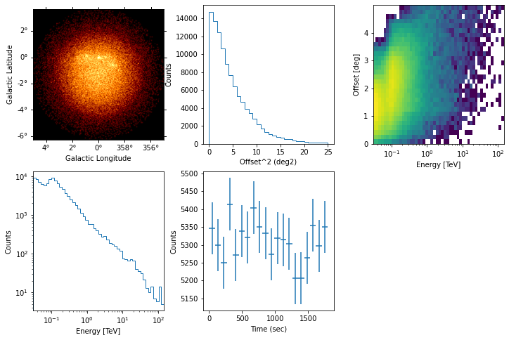
The quick-look events.peek() plot below shows that CTA has a field of view of a few degrees, and two energy thresholds, one significantly below 100 GeV where the CTA large-size telescopes (LSTs) detect events, and a second one near 100 GeV where the mid-sized telescopes (MSTs) start to detect events.

Note that most events are “hadronic background” due to cosmic ray showers in the atmosphere that pass the gamma-hadron selection cuts for this analysis configuration. Since this is simulated data, column MC_ID is available that gives an emission component identifier code, and the EVENTS header in events.table.meta can be used to look up which MC_ID corresponds to which emission component.

[13]:

events = observation.events
events

[13]:

<gammapy.data.event_list.EventList at 0x129638280>

[14]:

events = EventList.read(
    "$GAMMAPY_DATA/cta-1dc/data/baseline/gps/gps_baseline_110380.fits"
)
events

[14]:

<gammapy.data.event_list.EventList at 0x129602550>

[15]:

events.table[:5]

[15]:

Table length=5

EVENT_ID	TIME	RA	DEC	ENERGY	DETX	DETY	MC_ID
	s	deg	deg	TeV	deg	deg
uint32	float64	float32	float32	float32	float32	float32	int32
1	664502403.0454683	-92.63541	-30.514854	0.03902182	-0.9077294	-0.2727693	2
2	664502405.2579999	-92.64103	-28.262728	0.030796371	1.3443842	-0.2838398	2
3	664502408.8205513	-93.20372	-28.599625	0.04009629	1.0049409	-0.7769775	2
4	664502409.0143764	-94.03383	-29.269627	0.039580025	0.32684833	-1.496021	2
5	664502414.8090746	-93.330505	-30.319725	0.03035851	-0.716062	-0.8733348	2

[16]:

events.peek()

../../_images/tutorials_data_cta_22_0.png

IRFs¶

The CTA instrument response functions (IRFs) are given as FITS files in the caldb folder, the following IRFs are available:

effective area
energy dispersion
point spread function
background

Notes:

The IRFs contain the energy and offset dependence of the CTA response
CTA 1DC was based on an early version of the CTA FITS responses produced in 2017, improvements have been made since.
The point spread function was approximated by a Gaussian shape
The background is from hadronic and electron air shower events that pass CTA selection cuts. It was given as a function of field of view coordinates, although it is radially symmetric.
The energy dispersion in CTA 1DC is noisy at low energy, leading to unreliable spectral points for some analyses.
The CTA 1DC response files have the first node at field of view offset 0.5 deg, so to get the on-axis response at offset 0 deg, Gammapy has to extrapolate. Furthermore, because diffuse gamma-rays in the FOV were used to derive the IRFs, and the solid angle at small FOV offset circles is small, the IRFs at the center of the FOV are somewhat noisy. This leads to unstable analysis and simulation issues when using the DC1 IRFs for some analyses.

[17]:

observation.aeff

[17]:

<gammapy.irf.effective_area.EffectiveAreaTable2D at 0x13f462e80>

[18]:

irf_filename = (
    "$GAMMAPY_DATA/cta-1dc/caldb/data/cta/1dc/bcf/South_z20_50h/irf_file.fits"
)
irfs = load_cta_irfs(irf_filename)
irfs

Invalid unit found in background table! Assuming (s-1 MeV-1 sr-1)

[18]:

{'aeff': <gammapy.irf.effective_area.EffectiveAreaTable2D at 0x1299c4610>,
 'bkg': <gammapy.irf.background.Background3D at 0x13f494d60>,
 'edisp': <gammapy.irf.edisp.core.EnergyDispersion2D at 0x13f462b80>,
 'psf': <gammapy.irf.psf.parametric.EnergyDependentMultiGaussPSF at 0x13f494070>}

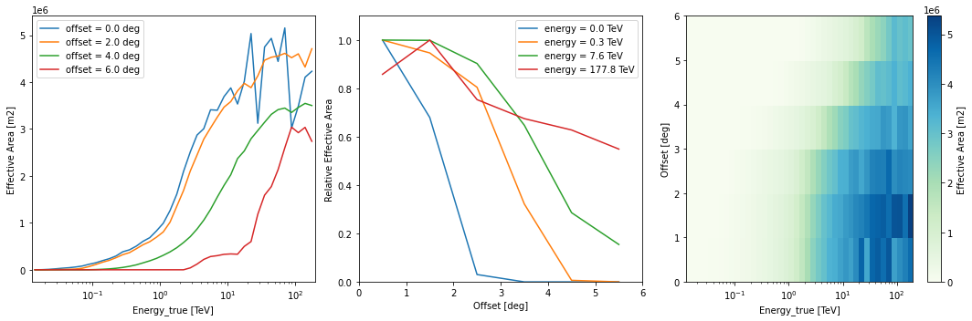
Effective area¶

[19]:

# Equivalent alternative way to load IRFs directly
aeff = EffectiveAreaTable2D.read(irf_filename, hdu="EFFECTIVE AREA")
aeff

[19]:

<gammapy.irf.effective_area.EffectiveAreaTable2D at 0x13f494490>

[20]:

irfs["aeff"].peek()

../../_images/tutorials_data_cta_28_0.png

[21]:

# What is the on-axis effective area at 10 TeV?
aeff.evaluate(energy_true="10 TeV", offset="0 deg").to("km2")

[21]:

$$3.783587 \; \mathrm{km^{2}}$$

Energy dispersion¶

[22]:

irfs["edisp"].peek()

../../_images/tutorials_data_cta_31_0.png

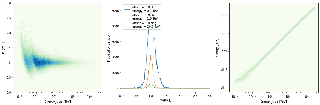
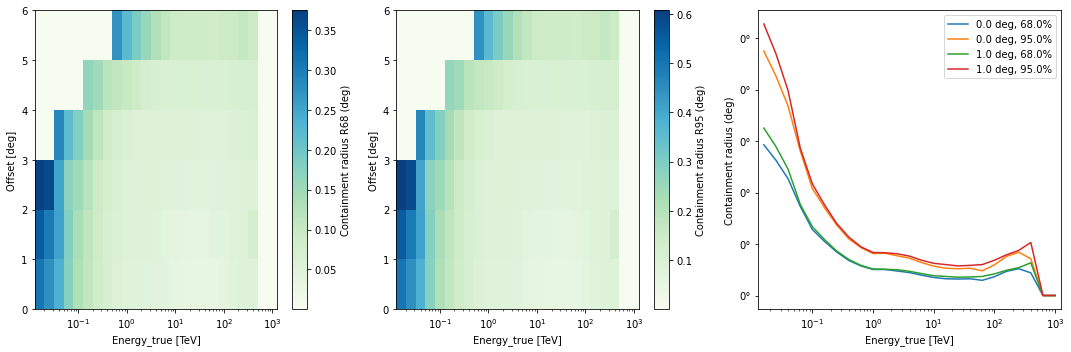
Point spread function¶

[23]:

irfs["psf"].peek()

../../_images/tutorials_data_cta_33_0.png

[24]:

# This is how for analysis you could slice out the PSF
# at a given field of view offset
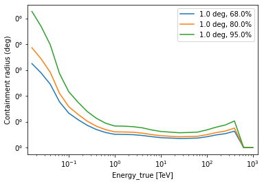
irfs["psf"].plot_containment_radius_vs_energy(
    offset=[1] * u.deg, fraction=[0.68, 0.8, 0.95]
);

../../_images/tutorials_data_cta_34_0.png

Background¶

The background is given as a rate in units MeV-1 s-1 sr-1.

[25]:

irfs["bkg"].peek()

../../_images/tutorials_data_cta_36_0.png

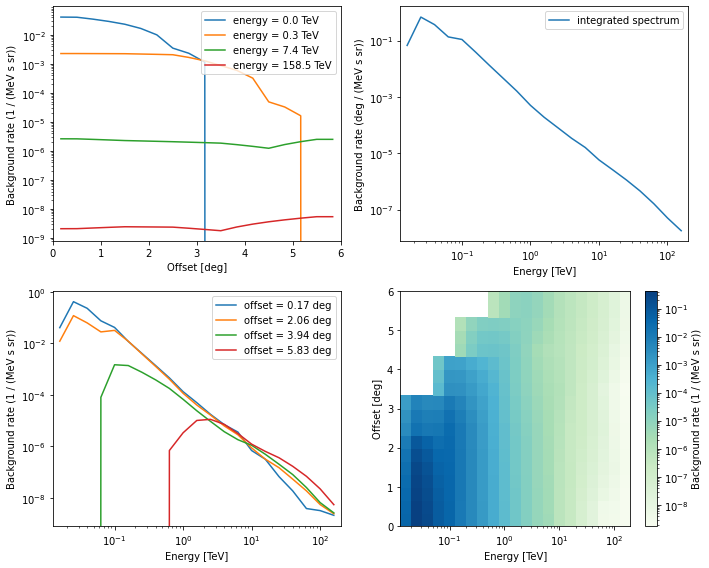
[26]:

irfs["bkg"].evaluate(energy="3 TeV", fov_lon="1 deg", fov_lat="0 deg")

[26]:

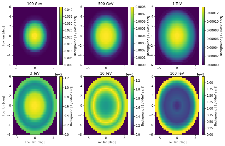
$$1.2053318 \times 10^{-5} \; \mathrm{\frac{1}{MeV\,s\,sr}}$$

To visualise the background at particular energies:

[27]:

irfs["bkg"].plot_at_energy(
    ["100 GeV", "500 GeV", "1 TeV", "3 TeV", "10 TeV", "100 TeV"]
)

../../_images/tutorials_data_cta_39_0.png

Source models¶

The 1DC sky model is distributed as a set of XML files, which in turn link to a ton of other FITS and text files. Gammapy doesn’t support this XML model file format. We are currently developing a YAML based format that improves upon the XML format, to be easier to write and read, add relevant information (units for physical quantities), and omit useless information (e.g. parameter scales in addition to values).

If you must or want to read the XML model files, you can use e.g. ElementTree from the Python standard library, or xmltodict if you pip install xmltodict. Here’s an example how to load the information for a given source, and to convert it into the sky model format Gammapy understands.

[28]:

# This is what the XML file looks like
# !tail -n 20 $CTADATA/models/models_gps.xml

[29]:

# TODO: write this example!

# Read XML file and access spectrum parameters
# from gammapy.extern import xmltodict

# filename = os.path.join(os.environ["CTADATA"], "models/models_gps.xml")
# data = xmltodict.parse(open(filename).read())
# data = data["source_library"]["source"][-1]
# data = data["spectrum"]["parameter"]
# data

[30]:

# Create a spectral model the the right units
# from astropy import units as u
# from gammapy.modeling.models import PowerLawSpectralModel

# par_to_val = lambda par: float(par["@value"]) * float(par["@scale"])
# spec = PowerLawSpectralModel(
#     amplitude=par_to_val(data[0]) * u.Unit("cm-2 s-1 MeV-1"),
#     index=par_to_val(data[1]),
#     reference=par_to_val(data[2]) * u.Unit("MeV"),
# )
# print(spec)

CTA performance files¶

CTA 1DC is useful to learn how to analyse CTA data. But to do simulations and studies for CTA now, you should get the most recent CTA IRFs in FITS format from https://www.cta-observatory.org/science/cta-performance/

If you want to run the download and examples in the next code cells, remove the # to uncomment.

[31]:

# !curl -O https://www.cta-observatory.org/wp-content/uploads/2019/04/CTA-Performance-prod3b-v2-FITS.tar.gz

[32]:

# !tar xf CTA-Performance-prod3b-v2-FITS.tar.gz

[33]:

# !ls caldb/data/cta/prod3b-v2/bcf

[34]:

# irfs1 = load_cta_irfs("caldb/data/cta/prod3b-v2/bcf/South_z20_50h/irf_file.fits")
# irfs1["aeff"].plot_energy_dependence()

[35]:

# irfs2 = load_cta_irfs("caldb/data/cta/prod3b-v2/bcf/South_z40_50h/irf_file.fits")
# irfs2["aeff"].plot_energy_dependence()

Exercises¶

Load the EVENTS file for obs_id=111159 as a gammapy.data.EventList object.
Use events.table to find the energy, sky coordinate and time of the highest-energy envent.
Use events.pointing_radec to find the pointing position of this observation, and use astropy.coordinates.SkyCoord methods to find the field of view offset of the highest-energy event.
What is the effective area and PSF 68% containment radius of CTA at 1 TeV for the South_z20_50h configuration used for the CTA 1DC simulation?
Get the latest CTA FITS performance files from https://www.cta-observatory.org/science/cta-performance/ and run the code example above. Make an effective area ratio plot of 40 deg zenith versus 20 deg zenith for the South_z40_50h and South_z20_50h configurations.

[36]:

# start typing here ...

Next steps¶

Learn how to analyse data with analysis_1.ipynb and analysis_2.ipynb or any other Gammapy analysis tutorial.
Learn how to evaluate CTA observability and sensitivity with simulate_3d.ipynb, spectrum_simulation.ipynb or cta_sensitivity.ipynb

[ ]: