Disk spatial model

This is a spatial model parametrising a disk.

By default, the model is symmetric, i.e. a disk:

\[\phi(lon, lat) = \frac{1}{2 \pi (1 - \cos{r_0}) } \cdot \begin{cases} 1 & \text{for } \theta \leq r_0 \ 0 & \text{for } \theta > r_0 \end{cases}\]

where \(\theta\) is the sky separation. To improve fit convergence of the model, the sharp edges is smoothed using erf.

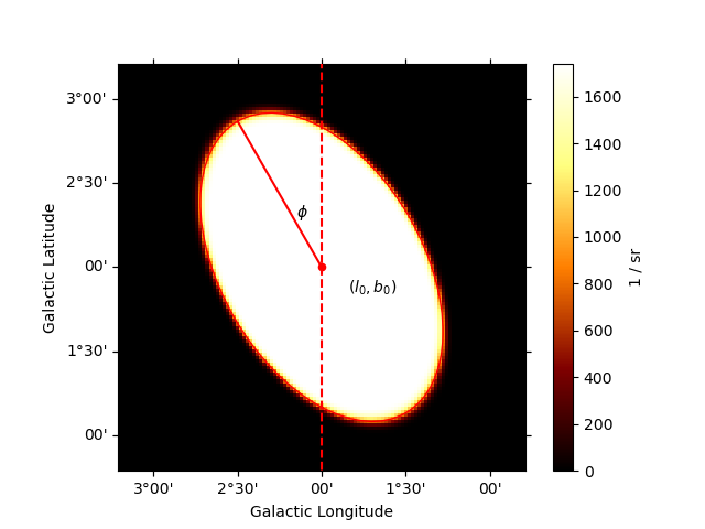
In case an eccentricity (e) and rotation angle (\(\phi\)) are passed, then the model is an elongated disk (i.e. an ellipse), with a major semiaxis of length \(r_0\) and position angle \(\phi\) (increasing counter-clockwise from the North direction).

The model is defined on the celestial sphere, with a normalization defined by:

\[\int_{4\pi}\phi(\text{lon}, \text{lat}) \,d\Omega = 1\,.\]

Example plot

Here is an example plot of the model:

import numpy as np
from astropy.coordinates import Angle
from gammapy.modeling.models import (
    DiskSpatialModel,
    Models,
    PowerLawSpectralModel,
    SkyModel,
)

phi = Angle("30 deg")
model = DiskSpatialModel(
    lon_0="2 deg",
    lat_0="2 deg",
    r_0="1 deg",
    e=0.8,
    phi=phi,
    edge_width=0.1,
    frame="galactic",
)

ax = model.plot(add_cbar=True)

# illustrate size parameter
region = model.to_region().to_pixel(ax.wcs)
artist = region.as_artist(facecolor="none", edgecolor="red")
ax.add_artist(artist)

transform = ax.get_transform("galactic")
ax.scatter(2, 2, transform=transform, s=20, edgecolor="red", facecolor="red")
ax.text(1.7, 1.85, r"$(l_0, b_0)$", transform=transform, ha="center")
ax.plot([2, 2 + np.sin(phi)], [2, 2 + np.cos(phi)], color="r", transform=transform)
ax.vlines(x=2, color="r", linestyle="--", transform=transform, ymin=0, ymax=5)
ax.text(2.15, 2.3, r"$\phi$", transform=transform)

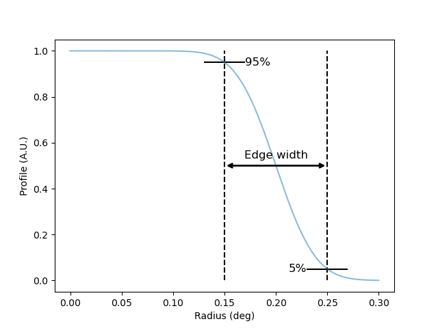
This plot illustrates the definition of the edge parameter:

import numpy as np
from astropy import units as u
from astropy.visualization import quantity_support
import matplotlib.pyplot as plt
from gammapy.modeling.models import DiskSpatialModel

lons = np.linspace(0, 0.3, 500) * u.deg

r_0, edge_width = 0.2 * u.deg, 0.5

disk = DiskSpatialModel(lon_0="0 deg", lat_0="0 deg", r_0=r_0, edge_width=edge_width)
profile = disk(lons, 0 * u.deg)

plt.plot(lons, profile / profile.max(), alpha=0.5)
plt.xlabel("Radius (deg)")
plt.ylabel("Profile (A.U.)")

edge_min, edge_max = r_0 * (1 - edge_width / 2.0), r_0 * (1 + edge_width / 2.0)
with quantity_support():
    plt.vlines([edge_min, edge_max], 0, 1, linestyles=["--"], color="k")
    plt.annotate(
        "",
        xy=(edge_min, 0.5),
        xytext=(edge_min + r_0 * edge_width, 0.5),
        arrowprops=dict(arrowstyle="<->", lw=2),
    )
    plt.text(0.2, 0.53, "Edge width", ha="center", size=12)
    margin = 0.02 * u.deg
    plt.hlines(
        [0.95], edge_min - margin, edge_min + margin, linestyles=["-"], color="k"
    )
    plt.text(edge_min + margin, 0.95, "95%", size=12, va="center")
    plt.hlines(
        [0.05], edge_max - margin, edge_max + margin, linestyles=["-"], color="k"
    )
    plt.text(edge_max - margin, 0.05, "5%", size=12, va="center", ha="right")
    plt.show()

YAML representation

Here is an example YAML file using the model:

pwl = PowerLawSpectralModel()
gauss = DiskSpatialModel()

model = SkyModel(spectral_model=pwl, spatial_model=gauss, name="pwl-disk-model")
models = Models([model])

print(models.to_yaml())

Out:

components:
-   name: pwl-disk-model
    type: SkyModel
    spectral:
        type: PowerLawSpectralModel
        parameters:
        -   name: index
            value: 2.0
        -   name: amplitude
            value: 1.0e-12
            unit: cm-2 s-1 TeV-1
        -   name: reference
            value: 1.0
            unit: TeV
            frozen: true
    spatial:
        type: DiskSpatialModel
        frame: icrs
        parameters:
        -   name: lon_0
            value: 0.0
            unit: deg
        -   name: lat_0
            value: 0.0
            unit: deg
        -   name: r_0
            value: 1.0
            unit: deg
        -   name: e
            value: 0.0
            frozen: true
        -   name: phi
            value: 0.0
            unit: deg
            frozen: true
        -   name: edge_width
            value: 0.01
            frozen: true