Note
Go to the end to download the full example code or to run this example in your browser via Binder.
Simulating and fitting a time varying source#
Simulate and fit a time decaying light curve of a source using the CTA 1DC response.
Prerequisites#
To understand how a single binned simulation works, please refer to 1D spectrum simulation tutorial and 3D map simulation tutorial for 1D and 3D simulations, respectively.
For details of light curve extraction using gammapy, refer to the two tutorials Light curves and Light curves for flares.
Context#
Frequently, studies of variable sources (eg: decaying GRB light curves, AGN flares, etc.) require time variable simulations. For most use cases, generating an event list is an overkill, and it suffices to use binned simulations using a temporal model.
Objective: Simulate and fit a time decaying light curve of a source with CTA using the CTA 1DC response.
Proposed approach#
We will simulate 10 spectral datasets within given time intervals (Good Time Intervals) following a given spectral (a power law) and temporal profile (an exponential decay, with a decay time of 6 hr). These are then analysed using the light curve estimator to obtain flux points.
Modelling and fitting of lightcurves can be done either - directly on
the output of the LightCurveEstimator (at the DL5 level) - fit the
simulated datasets (at the DL4 level)
In summary, the necessary steps are:
Choose observation parameters including a list of
gammapy.data.GTIDefine temporal and spectral models from the Model gallery as per science case
Perform the simulation (in 1D or 3D)
Extract the light curve from the reduced dataset as shown in Light curves tutorial
Optionally, we show here how to fit the simulated datasets using a source model
Setup#
As usual, we’ll start with some general imports…
import logging
import numpy as np
import astropy.units as u
from astropy.coordinates import SkyCoord
from astropy.time import Time

# %matplotlib inline
import matplotlib.pyplot as plt
from IPython.display import display

log = logging.getLogger(__name__)
And some gammapy specific imports
import warnings
from gammapy.data import FixedPointingInfo, Observation, observatory_locations
from gammapy.datasets import Datasets, FluxPointsDataset, SpectrumDataset
from gammapy.estimators import LightCurveEstimator
from gammapy.irf import load_irf_dict_from_file
from gammapy.makers import SpectrumDatasetMaker
from gammapy.maps import MapAxis, RegionGeom, TimeMapAxis
from gammapy.modeling import Fit
from gammapy.modeling.models import (
    ExpDecayTemporalModel,
    PowerLawSpectralModel,
    SkyModel,
)

warnings.filterwarnings(
    action="ignore", message="overflow encountered in exp", module="astropy"
)
We first define our preferred time format:
TimeMapAxis.time_format = "iso"
Simulating a light curve#
We will simulate 10 spectra between 300 GeV and 10 TeV using an
PowerLawSpectralModel and a
ExpDecayTemporalModel. The important
thing to note here is how to attach a different GTI to each dataset.
Since we use spectrum datasets here, we will use a RegionGeom.
# Loading IRFs
irfs = load_irf_dict_from_file(
    "$GAMMAPY_DATA/cta-1dc/caldb/data/cta/1dc/bcf/South_z20_50h/irf_file.fits"
)

# Reconstructed and true energy axis
energy_axis = MapAxis.from_edges(
    np.logspace(-0.5, 1.0, 10), unit="TeV", name="energy", interp="log"
)
energy_axis_true = MapAxis.from_edges(
    np.logspace(-1.2, 2.0, 31), unit="TeV", name="energy_true", interp="log"
)

geom = RegionGeom.create("galactic;circle(0, 0, 0.11)", axes=[energy_axis])

# Pointing position to be supplied as a `FixedPointingInfo`
pointing = FixedPointingInfo(
    fixed_icrs=SkyCoord(0.5, 0.5, unit="deg", frame="galactic").icrs,
)
/home/runner/work/gammapy-docs/gammapy-docs/gammapy/.tox/build_docs/lib/python3.12/site-packages/astropy/units/core.py:2102: UnitsWarning: '1/s/MeV/sr' did not parse as fits unit: Numeric factor not supported by FITS If this is meant to be a custom unit, define it with 'u.def_unit'. To have it recognized inside a file reader or other code, enable it with 'u.add_enabled_units'. For details, see https://docs.astropy.org/en/latest/units/combining_and_defining.html
  warnings.warn(msg, UnitsWarning)
Note that observations are usually conducted in Wobble mode, in which the source is not in the center of the camera. This allows to have a symmetrical sky position from which background can be estimated.
# Define the source model: A combination of spectral and temporal model

gti_t0 = Time("2020-03-01")
spectral_model = PowerLawSpectralModel(
    index=3, amplitude="1e-11 cm-2 s-1 TeV-1", reference="1 TeV"
)
temporal_model = ExpDecayTemporalModel(t0="6 h", t_ref=gti_t0.mjd * u.d)

model_simu = SkyModel(
    spectral_model=spectral_model,
    temporal_model=temporal_model,
    name="model-simu",
)

# Look at the model
display(model_simu.parameters.to_table())
type    name     value         unit        error   min max frozen link prior
---- --------- ---------- -------------- --------- --- --- ------ ---- -----
         index 3.0000e+00                0.000e+00 nan nan  False
     amplitude 1.0000e-11 TeV-1 s-1 cm-2 0.000e+00 nan nan  False
     reference 1.0000e+00            TeV 0.000e+00 nan nan   True
            t0 6.0000e+00              h 0.000e+00 nan nan  False
         t_ref 5.8909e+04              d 0.000e+00 nan nan   True
Now, define the start and observation livetime wrt to the reference
time, gti_t0
Now perform the simulations
datasets = Datasets()

empty = SpectrumDataset.create(
    geom=geom, energy_axis_true=energy_axis_true, name="empty"
)

maker = SpectrumDatasetMaker(selection=["exposure", "background", "edisp"])


for idx in range(n_obs):
    obs = Observation.create(
        pointing=pointing,
        livetime=lvtm[idx],
        tstart=tstart[idx],
        irfs=irfs,
        reference_time=gti_t0,
        obs_id=idx,
        location=observatory_locations["ctao_south"],
    )
    empty_i = empty.copy(name=f"dataset-{idx}")
    dataset = maker.run(empty_i, obs)
    dataset.models = model_simu
    dataset.fake()
    datasets.append(dataset)
The reduced datasets have been successfully simulated. Let’s take a quick look into our datasets.
display(datasets.info_table())
   name   counts       excess       ... n_fit_bins stat_type       stat_sum
                                    ...
--------- ------ ------------------ ... ---------- --------- -------------------
dataset-0    787  766.6812310184489 ...          9      cash -6219.2830448037475
dataset-1    333 323.76419591747674 ...          9      cash   -2081.44633285044
dataset-2    298  288.3947637541758 ...          9      cash -1758.5527342970606
dataset-3    318  303.2227134679628 ...          9      cash -1919.6523864690353
dataset-4    190 175.22271346796282 ...          9      cash  -920.6036961739541
dataset-5    175 156.52839183495354 ...          9      cash  -872.0639130761929
dataset-6     43 28.222713467962826 ...          9      cash  -87.88022487138169
dataset-7     35  15.78952750835169 ...          9      cash  -41.25685534627986
dataset-8     33 17.114416978060042 ...          9      cash  -52.64025949689469
dataset-9     21 3.6366883248563298 ...          9      cash -16.445007146304523
Extract the lightcurve#
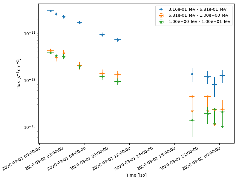
This section uses standard light curve estimation tools for a 1D extraction. Only a spectral model needs to be defined in this case. Since the estimator returns the integrated flux separately for each time bin, the temporal model need not be accounted for at this stage. We extract the lightcurve in 3 energy bins.
# Define the model:
spectral_model = PowerLawSpectralModel(
    index=3, amplitude="1e-11 cm-2 s-1 TeV-1", reference="1 TeV"
)
model_fit = SkyModel(spectral_model=spectral_model, name="model-fit")

# Attach model to all datasets
datasets.models = model_fit

lc_maker_1d = LightCurveEstimator(
    energy_edges=[0.3, 0.6, 1.0, 10] * u.TeV,
    source="model-fit",
    selection_optional=["ul"],
)
lc_1d = lc_maker_1d.run(datasets)

fig, ax = plt.subplots(
    figsize=(8, 6),
    gridspec_kw={"left": 0.16, "bottom": 0.2, "top": 0.98, "right": 0.98},
)
lc_1d.plot(ax=ax, marker="o", axis_name="time", sed_type="flux")
plt.show()
Fitting temporal models#
We have the reconstructed lightcurve at this point. Now we want to fit a profile to the obtained light curves, using a joint fitting across the different datasets, while simultaneously minimising across the temporal model parameters as well. The temporal models can be applied
directly on the obtained lightcurve
on the simulated datasets
Fitting the obtained light curve#
We will first convert the obtained light curve to a FluxPointsDataset
and fit it with a spectral and temporal model
# Create the datasets by iterating over the returned lightcurve
dataset_fp = FluxPointsDataset(data=lc_1d, name="dataset_lc")
We will fit the amplitude, spectral index and the decay time scale. Note
that t_ref should be fixed by default for the
ExpDecayTemporalModel.
# Define the model:
spectral_model1 = PowerLawSpectralModel(
    index=2.0, amplitude="1e-12 cm-2 s-1 TeV-1", reference="1 TeV"
)
temporal_model1 = ExpDecayTemporalModel(t0="10 h", t_ref=gti_t0.mjd * u.d)


model = SkyModel(
    spectral_model=spectral_model1,
    temporal_model=temporal_model1,
    name="model-test",
)

dataset_fp.models = model
print(dataset_fp)


# Fit the dataset
fit = Fit()
result = fit.run(dataset_fp)
display(result.parameters.to_table())
FluxPointsDataset
-----------------

  Name                            : dataset_lc

  Number of total flux points     : 30
  Number of fit bins              : 25

  Fit statistic type              : chi2
  Fit statistic value (-2 log(L)) : 1436.20

  Number of models                : 1
  Number of parameters            : 5
  Number of free parameters       : 3

  Component 0: SkyModel

    Name                      : model-test
    Datasets names            : None
    Spectral model type       : PowerLawSpectralModel
    Spatial  model type       :
    Temporal model type       : ExpDecayTemporalModel
    Parameters:
      index                         :      2.000   +/-    0.00
      amplitude                     :   1.00e-12   +/- 0.0e+00 1 / (TeV s cm2)
      reference             (frozen):      1.000       TeV
      t0                            :     10.000   +/-    0.00 h
      t_ref                 (frozen):  58909.000       d


type    name     value         unit        error   min max frozen link prior
---- --------- ---------- -------------- --------- --- --- ------ ---- -----
         index 2.9493e+00                2.749e-02 nan nan  False
     amplitude 9.8887e-12 TeV-1 s-1 cm-2 3.324e-13 nan nan  False
     reference 1.0000e+00            TeV 0.000e+00 nan nan   True
            t0 5.9004e+00              h 2.180e-01 nan nan  False
         t_ref 5.8909e+04              d 0.000e+00 nan nan   True
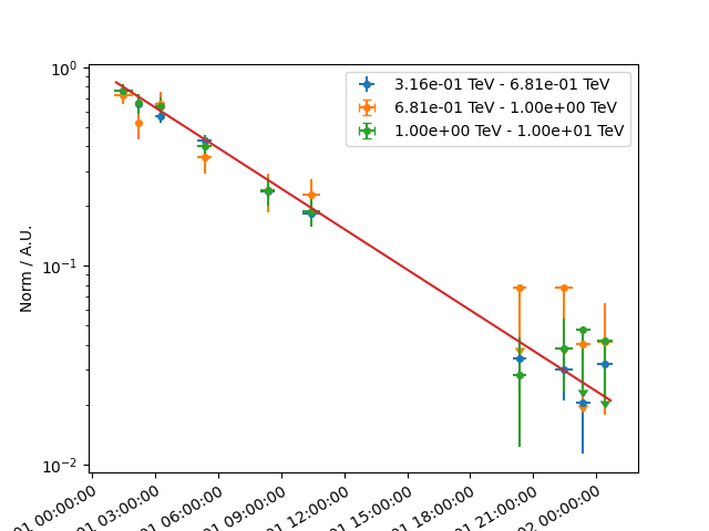
Now let’s plot model and data. We plot only the normalisation of the temporal model in relative units for one particular energy range
plt.figure(figsize=(8, 7))
plt.subplots_adjust(bottom=0.3)
dataset_fp.plot_spectrum(axis_name="time")
plt.show()
/home/runner/work/gammapy-docs/gammapy-docs/gammapy/.tox/build_docs/lib/python3.12/site-packages/gammapy/maps/region/ndmap.py:154: UserWarning: This axis already has a converter set and is updating to a potentially incompatible converter
  ax.errorbar(
Fit the datasets#
Here, we apply the models directly to the simulated datasets.
For modelling and fitting more complex flares, you should attach the
relevant model to each group of datasets. The parameters of a model
in a given group of dataset will be tied. For more details on joint
fitting in Gammapy, see the 3D detailed analysis.
# Define the model:
spectral_model2 = PowerLawSpectralModel(
    index=2.0, amplitude="1e-12 cm-2 s-1 TeV-1", reference="1 TeV"
)
temporal_model2 = ExpDecayTemporalModel(t0="10 h", t_ref=gti_t0.mjd * u.d)

model2 = SkyModel(
    spectral_model=spectral_model2,
    temporal_model=temporal_model2,
    name="model-test2",
)

display(model2.parameters.to_table())

datasets.models = model2

# Perform a joint fit
fit = Fit()
result = fit.run(datasets=datasets)

display(result.parameters.to_table())
type    name     value         unit        error   min max frozen link prior
---- --------- ---------- -------------- --------- --- --- ------ ---- -----
         index 2.0000e+00                0.000e+00 nan nan  False
     amplitude 1.0000e-12 TeV-1 s-1 cm-2 0.000e+00 nan nan  False
     reference 1.0000e+00            TeV 0.000e+00 nan nan   True
            t0 1.0000e+01              h 0.000e+00 nan nan  False
         t_ref 5.8909e+04              d 0.000e+00 nan nan   True
type    name     value         unit        error   min max frozen link prior
---- --------- ---------- -------------- --------- --- --- ------ ---- -----
         index 2.9274e+00                3.127e-02 nan nan  False
     amplitude 1.0166e-11 TeV-1 s-1 cm-2 3.511e-13 nan nan  False
     reference 1.0000e+00            TeV 0.000e+00 nan nan   True
            t0 5.8394e+00              h 2.017e-01 nan nan  False
         t_ref 5.8909e+04              d 0.000e+00 nan nan   True
We see that the fitted parameters are consistent between fitting flux points and datasets, and match well with the simulated ones
Exercises#
Re-do the analysis with
MapDatasetinstead of aSpectrumDatasetModel the flare of PKS 2155-304 which you obtained using the Light curves for flares tutorial. Use a combination of a Gaussian and Exponential flare profiles.
Do a joint fitting of the datasets.
Total running time of the script: (0 minutes 15.044 seconds)