Computing flux upper limits

Explore how to compute flux upper limits for a non-detected source.

Prerequisites

It is advisable to understand the general Gammapy modeling and fitting framework before proceeding with this notebook, e.g. Modeling and Fitting (DL4 to DL5).

Context

In the study of VHE sources, one often encounters no significant detection even after long exposures. In that case, it may be useful to compute flux upper limits (UL) for the said target consistent with the observation.

Proposed approach

In this section, we will use an empty observation from the H.E.S.S. DL3 DR1 to understand how to quantify non-detections. There are two distinct approaches to consider:

• Test for the presence of emission anywhere in a map and compute an integral flux upper limit at any position (i.e. UL map).

• Test the presence of emission from a potential source with given position and morphology and compute integral and differential UL

Setup

As usual, let’s start with some general imports…

# %matplotlib inline
import matplotlib.pyplot as plt

import astropy.units as u

from gammapy.datasets import MapDataset, Datasets
from gammapy.estimators import FluxPointsEstimator, ExcessMapEstimator
from gammapy.modeling import select_nested_models
from gammapy.modeling.models import (
    PointSpatialModel,
    PowerLawSpectralModel,
    SkyModel,
    create_crab_spectral_model,
)
from gammapy.visualization import plot_distribution

Load observation

For computational purposes, we have already created a MapDataset from observation id 20275 from the public H.E.S.S. data release and stored it in $GAMMAPY_DATA

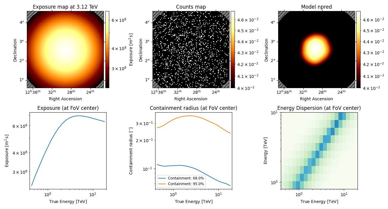
dataset = MapDataset.read("$GAMMAPY_DATA/datasets/empty-dl4/empty-dl4.fits.gz")
dataset.peek()
plt.show()

Create Upper Limit maps

We will first use the ExcessMapEstimator for a quick check to see if there are any potential sources in the field. The correlation_radius should be around the size of the source you are searching for. You may also use the TSMapEstimator.

estimator = ExcessMapEstimator(
    sum_over_energy_groups=True,
    selection_optional="all",
    correlate_off=True,
    correlation_radius=0.1 * u.deg,
)

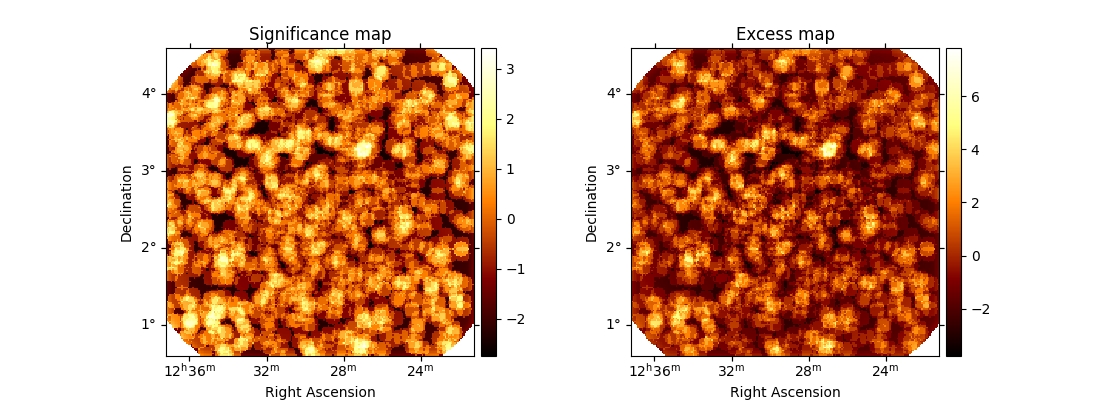
lima_maps = estimator.run(dataset)

significance_map = lima_maps["sqrt_ts"]
excess_map = lima_maps["npred_excess"]

fig, (ax1, ax2) = plt.subplots(
    figsize=(11, 4), subplot_kw={"projection": lima_maps.geom.wcs}, ncols=2
)
ax1.set_title("Significance map")
significance_map.plot(ax=ax1, add_cbar=True)
ax2.set_title("Excess map")
excess_map.plot(ax=ax2, add_cbar=True)
plt.show()

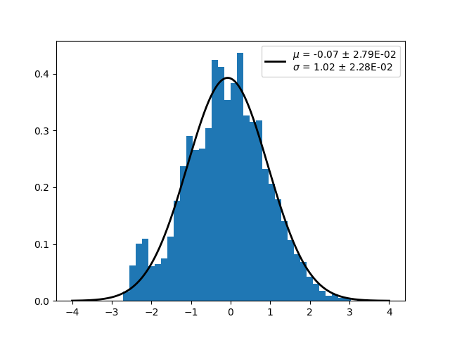
The significance map looks featureless. We will plot a histogram of the significance distribution and fit it with a standard normal. Deviations from a standard normal can suggest the presence of gamma-ray sources, or can also originate from incorrect modeling of the residual hadronic background.

ax = plt.subplot()
plot_distribution(
    significance_map,
    func="norm",
    ax=ax,
    kwargs_hist={"bins": 50, "range": (-4, 4), "density": True},
)
plt.show()

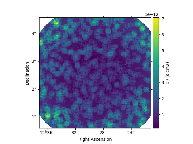
We can also see the correlated upper limits at any position in the map. However, it is important to note that this is not a source UL, as the containment correction is not applied here. Instead, it gives the flux upper limits contained within the correlation_radius at each pixel. This can be useful when making quick look plots to search for the presence of new sources with a field - for example in the case of alerts from Gravitational Wave detectors.

lima_maps.flux_ul.plot(add_cbar=True, cmap="viridis")
plt.show()

Compute upper limits for a source

Now, we address a more specific question. Suppose we were expecting a source at a specific position, say the center of our map. We’ll attempt to fit a point source at that location to determine whether the signal is significant above the background.

For this, we compare two hypotheses:

• Null hypothesis, \(H_0\) - only the background is present (i.e., no source)

• Alternative hypothesis, \(H_1\) - the background plus a point source

The difference in test statistic (TS) between the two cases indicates the significance of the alternative hypothesis.

For this purpose, we can utilise the function select_nested_models which performs these comparisons internally. As the null hypothesis, \(H_0\), corresponds to the case of no source, we set the amplitude to 0, in other words the source has no flux.

To prevent the fit from converging to unrelated positions, we freeze the spatial parameters. Alternatively, you can constrain the parameter ranges to stay within your expected region.

spectral_model = PowerLawSpectralModel()
spatial_model = PointSpatialModel(lon_0=187 * u.deg, lat_0=2.6 * u.deg, frame="icrs")
spatial_model.lat_0.frozen = True
spatial_model.lon_0.frozen = True

sky_model = SkyModel(
    spatial_model=spatial_model, spectral_model=spectral_model, name="source"
)
dataset.models = sky_model
LLR = select_nested_models(
    datasets=Datasets(dataset),
    parameters=[sky_model.parameters["amplitude"]],
    null_values=[0],
)
print(LLR)

{'ts': 4.583718379990387, 'fit_results': <gammapy.modeling.fit.FitResult object at 0x7fd5e072d790>, 'fit_results_null': <gammapy.modeling.fit.FitResult object at 0x7fd5be0f8f50>}

The fitted parameters under the alternative hypothesis:

print(LLR["fit_results"].parameters.to_table())

type    name      value         unit      ...    max    frozen link prior
---- --------- ----------- -------------- ... --------- ------ ---- -----
         index  1.1760e+00                ...       nan  False
     amplitude -8.4167e-13 TeV-1 s-1 cm-2 ...       nan  False
     reference  1.0000e+00            TeV ...       nan   True
         lon_0  1.8700e+02            deg ...       nan   True
         lat_0  2.6000e+00            deg ... 9.000e+01   True

The test statistic is ts ~ 4.7. Note that here we have only 1 free parameter, the amplitude, and thus, we can assume the simple conversion significance = \(\sqrt{ts} \approx 2.2\). Therefore, the observed fluctuations are not significant above the background. Next, we will estimate the differential upper limits of the source.

Differential upper limits

In the absence of a detection, using the model directly from the fit is meaningless as its features can be simply due to background fluctuations. It is important to set a reasonable model on the dataset before proceeding with the FluxPointsEstimator. This model can come from measurements from other instruments, be an extrapolation of the flux observed at other wavelengths, come from theoretical estimations, etc. In particular, a model with a negative amplitude as obtained above should not be used.

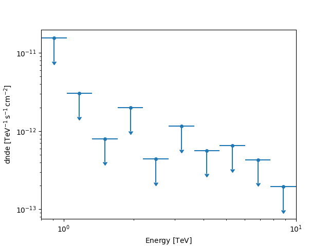
Note that the computed upper limits depend on the spectral parameters of the assumed model. Here, we compute the 3-sigma upper limits for assuming a spectral index of 2.0. We also fix the spatial parameters of the model to prevent the minimiser from wandering off to different regions in the FoV.

sky_model.parameters["amplitude"].value = 1e-14
sky_model.parameters["index"].value = 2.0
sky_model.freeze(model_type="spatial")

energy_edges = dataset.geoms["geom"].axes["energy"].edges
fpe = FluxPointsEstimator(
    selection_optional="all",
    energy_edges=energy_edges,
    n_sigma_ul=3,
    source="source",
)

fp1 = fpe.run(dataset)


fp1.plot(sed_type="dnde")
plt.show()

Integral upper limits

To compute the integral upper limits between certain energies, we can simply run FluxPointsEstimator with one bin in energy.

emin = energy_edges[0]
emax = energy_edges[-1]
fpe2 = FluxPointsEstimator(
    selection_optional=["ul"], energy_edges=[emin, emax], source="source"
)
fp2 = fpe2.run(dataset)
print(
    f"Integral upper limit between {emin:.1f} and {emax:.1f} is {fp2.flux_ul.quantity.ravel()[0]:.2e}"
)

Integral upper limit between 0.8 TeV and 10.0 TeV is 7.76e-14 1 / (s cm2)

Sensitivity estimation

We can then ask, would this source have been detectable given this IRF/exposure time?

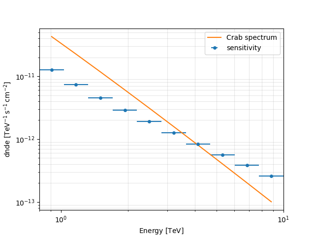
The FluxPointsEstimator can be used to obtain the sensitivity, which can be compared to the flux prediction for a given (hypothetical) source. We have the 5-sigma sensitivity here, which can be configured using n_sigma_sensitivity parameter of this estimator. Let us see what we would have seen if a Crab-like source was present in the center. Note that this computed sensitivity does not take into account the factors such as the minimum number of gamma-rays (see Point source sensitivity) and is dependent on the analysis configuration. We compare this with the known Crab spectrum.

crab_model = create_crab_spectral_model()

fp1.dnde_sensitivity.plot(label="sensitivity")
crab_model.plot(
    energy_bounds=fp1.geom.axes["energy"], sed_type="dnde", label="Crab spectrum"
)
plt.grid(which="minor", alpha=0.3)

plt.legend()
plt.show()

Thus, a Crab-like source should have been above our sensitivity till around ~ 4 TeV for this specific observation.