Note
Go to the end to download the full example code or to run this example in your browser via Binder.
Data structures#
Introduction to basic data structures handling.
Introduction#
This is a getting started tutorial for Gammapy.
In this tutorial we will use the Third Fermi-LAT Catalog of High-Energy Sources (3FHL) catalog, corresponding event list and images to learn how to work with some of the central Gammapy data structures.
We will cover the following topics:
Sky maps
Event lists
Source catalogs
We will show how to load source catalogs with Gammapy and explore the data using the following classes:
SourceCatalog, specificallySourceCatalog3FHL
Spectral models and flux points
We will pick an example source and show how to plot its spectral model and flux points. For this we will use the following classes:
SpectralModel, specifically thePowerLaw2SpectralModel
Setup#
Important: to run this tutorial the environment variable
GAMMAPY_DATA must be defined and point to the directory on your
machine where the datasets needed are placed. To check whether your
setup is correct you can execute the following cell:
import astropy.units as u
from astropy.coordinates import SkyCoord
import matplotlib.pyplot as plt
Check setup#
from gammapy.utils.check import check_tutorials_setup

# %matplotlib inline


check_tutorials_setup()
System:

        python_executable      : /home/runner/work/gammapy-docs/gammapy-docs/gammapy/.tox/build_docs/bin/python
        python_version         : 3.12.13
        machine                : x86_64
        system                 : Linux


Gammapy package:

        version                : 2.0.dev4000+g6ed4106cb
        path                   : /home/runner/work/gammapy-docs/gammapy-docs/gammapy/.tox/build_docs/lib/python3.12/site-packages/gammapy


Other packages:

        numpy                  : 2.4.6
        scipy                  : 1.17.1
        astropy                : 7.2.2
        regions                : 0.11
        click                  : 8.4.2
        PyYAML                 : 6.0.3
        pydantic               : 2.13.4
        IPython                : 9.15.0
        jupyter                : not installed
        jupyterlab             : not installed
        matplotlib             : 3.11.1
        pandas                 : 3.0.3
        healpy                 : 1.19.0
        iminuit                : 2.32.0
        sherpa                 : 4.18.0
        naima                  : 0.10.3
        emcee                  : 3.1.6
        corner                 : 2.3.0
        ray                    : 2.54.1


Gammapy environment variables:

        GAMMAPY_DATA           : /home/runner/work/gammapy-docs/gammapy-docs/gammapy-datasets/dev
Maps#
The maps package contains classes to work with sky images
and cubes.
In this section, we will use a simple 2D sky image and will learn how to:
Read sky images from FITS files
Smooth images
Plot images
Cutout parts from images
The image is a WcsNDMap object:
print(gc_3fhl)
WcsNDMap

        geom  : WcsGeom
        axes  : ['lon', 'lat']
        shape : (np.int64(400), np.int64(200))
        ndim  : 2
        unit  :
        dtype : >i8
The shape of the image is 400 x 200 pixel and it is defined using a cartesian projection in galactic coordinates.
The geom attribute is a WcsGeom object:
print(gc_3fhl.geom)
WcsGeom

        axes       : ['lon', 'lat']
        shape      : (np.int64(400), np.int64(200))
        ndim       : 2
        frame      : galactic
        projection : CAR
        center     : 0.0 deg, 0.0 deg
        width      : 20.0 deg x 10.0 deg
        wcs ref    : 0.0 deg, 0.0 deg
Let’s take a closer look at the .data attribute:
print(gc_3fhl.data)
[[0 0 0 ... 0 0 0]
 [0 0 0 ... 0 0 0]
 [0 0 0 ... 0 0 0]
 ...
 [0 0 0 ... 0 0 1]
 [0 0 0 ... 0 0 0]
 [0 0 0 ... 0 0 1]]
That looks familiar! It just an ordinary 2 dimensional numpy array, which means you can apply any known numpy method to it:
print(f"Total number of counts in the image: {gc_3fhl.data.sum():.0f}")
Total number of counts in the image: 32684
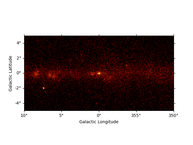
To show the image on the screen we can use the plot method. It
basically calls
plt.imshow,
passing the gc_3fhl.data attribute but in addition handles axis with
world coordinates using
astropy.visualization.wcsaxes
and defines some defaults for nicer plots (e.g. the colormap ‘afmhot’):
gc_3fhl.plot(stretch="sqrt")
plt.show()
To make the structures in the image more visible we will smooth the data using a Gaussian kernel.
gc_3fhl_smoothed = gc_3fhl.smooth(kernel="gauss", width=0.2 * u.deg)
gc_3fhl_smoothed.plot(stretch="sqrt")
plt.show()
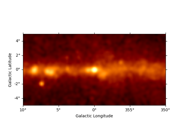
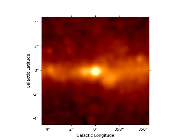
The smoothed plot already looks much nicer, but still the image is
rather large. As we are mostly interested in the inner part of the
image, we will cut out a quadratic region of the size 9 deg x 9 deg
around Vela. Therefore, we use cutout to make a
cutout map:
# define center and size of the cutout region
center = SkyCoord(0, 0, unit="deg", frame="galactic")
gc_3fhl_cutout = gc_3fhl_smoothed.cutout(center, 9 * u.deg)
gc_3fhl_cutout.plot(stretch="sqrt")
plt.show()
For a more detailed introduction to maps, take a look at the
Maps notebook.
Exercises#
Add a marker and circle at the position of Sgr A* (you can find examples in astropy.visualization.wcsaxes).
Event lists#
Almost any high level gamma-ray data analysis starts with the raw
measured counts data, which is stored in event lists. In Gammapy event
lists are represented by the EventList class.
In this section we will learn how to:
Read event lists from FITS files
Access and work with the
EventListattributes such as.tableand.energyFilter events lists using convenience methods
Let’s start with the import from the data submodule:
from gammapy.data import EventList
Very similar to the sky map class an event list can be created, by
passing a filename to the read() method:
events_3fhl = EventList.read("$GAMMAPY_DATA/fermi-3fhl-gc/fermi-3fhl-gc-events.fits.gz")
This time the actual data is stored as an Table
object. It can be accessed with .table attribute:
print(events_3fhl.table)
       TIME          ENERGY      RA       DEC     ... DIFRSP2 DIFRSP3 DIFRSP4
                      MeV       deg       deg     ...
------------------ --------- --------- ---------- ... ------- ------- -------
 54682.82946153034 12186.642 260.45935 -33.553337 ...     0.0     0.0     0.0
 54682.89243456219 25496.598 261.37506 -34.395004 ...     0.0     0.0     0.0
 54682.89709471887 15621.498 259.56973 -33.409416 ...     0.0     0.0     0.0
54683.217347750084  12816.32 273.95883 -25.340391 ...     0.0     0.0     0.0
54683.286774636625 18988.387  260.8568 -36.355804 ...     0.0     0.0     0.0
   54683.421513173  11610.23 266.15518 -26.224436 ...     0.0     0.0     0.0
 54683.54876572769 13960.802 271.44742 -29.615316 ...     0.0     0.0     0.0
 54683.55585722025 10477.372  266.3981  -28.96814 ...     0.0     0.0     0.0
 54683.61038647694  13030.88 271.70428 -20.632627 ...     0.0     0.0     0.0
               ...       ...       ...        ... ...     ...     ...     ...
57236.219039132106 387834.72  270.3779  -21.56711 ...     0.0     0.0     0.0
57236.225316976816  20559.74  268.5538 -26.345692 ...     0.0     0.0     0.0
 57236.28290302389 27209.146 266.59344  -30.52607 ...     0.0     0.0     0.0
 57236.36520195913 13911.061 269.30997 -27.239439 ...     0.0     0.0     0.0
57236.426843659276 13226.425 265.16287 -27.344238 ...     0.0     0.0     0.0
 57236.68330055816 17445.463 266.63342 -28.807201 ...     0.0     0.0     0.0
 57236.68695264887 13133.864 270.42474 -22.651058 ...     0.0     0.0     0.0
 57236.75267734621 32095.705  266.0002  -29.77206 ...     0.0     0.0     0.0
 57233.37455140838 18465.783 266.39728 -29.105953 ...     0.0     0.0     0.0
 57233.44802851667  14457.25 262.72217 -34.388405 ...     0.0     0.0     0.0
Length = 32843 rows
You can do len over event_3fhl.table to find the total number of
events.
print(len(events_3fhl.table))
32843
And we can access any other attribute of the Table object as well:
print(events_3fhl.table.colnames)
['TIME', 'ENERGY', 'RA', 'DEC', 'L', 'B', 'THETA', 'PHI', 'ZENITH_ANGLE', 'EARTH_AZIMUTH_ANGLE', 'EVENT_ID', 'RUN_ID', 'RECON_VERSION', 'CALIB_VERSION', 'EVENT_CLASS', 'EVENT_TYPE', 'CONVERSION_TYPE', 'LIVETIME', 'DIFRSP0', 'DIFRSP1', 'DIFRSP2', 'DIFRSP3', 'DIFRSP4']
For convenience we can access the most important event parameters as
properties on the EventList objects. The attributes will return
corresponding Astropy objects to represent the data, such as
Quantity, SkyCoord or
Time objects:
print(events_3fhl.energy.to("GeV"))
[12.186643 25.4966 15.621499 ... 32.095707 18.465784 14.457251] GeV
print(events_3fhl.galactic)
# events_3fhl.radec
<SkyCoord (Galactic): (l, b) in deg
    [(353.36228879,  1.75408483), (353.09562941,  0.6522806 ),
     (353.05628243,  2.44528685), ..., (359.10295505, -0.1359316 ),
     (359.85157506, -0.08269984), (353.71795506, -0.26883694)]>
print(events_3fhl.time)
[54682.82946153 54682.89243456 54682.89709472 ... 57236.75267735
 57233.37455141 57233.44802852]
In addition EventList provides convenience methods to filter the
event lists. One possible use case is to find the highest energy event
within a radius of 0.5 deg around the vela position:
# select all events within a radius of 0.5 deg around center
from gammapy.utils.regions import SphericalCircleSkyRegion

region = SphericalCircleSkyRegion(center, radius=0.5 * u.deg)
events_gc_3fhl = events_3fhl.select_region(region)

# sort events by energy
events_gc_3fhl.table.sort("ENERGY")

# and show highest energy photon
print("highest energy photon: ", events_gc_3fhl.energy[-1].to("GeV"))
highest energy photon: 1917.859375 GeV
Exercises#
Make a counts energy spectrum for the galactic center region, within a radius of 10 deg.
Source catalogs#
Gammapy provides a convenient interface to access and work with catalog based data.
In this section we will learn how to:
Load builtins catalogs from
catalogSort and index the underlying Astropy tables
Access data from individual sources
Let’s start with importing the 3FHL catalog object from the
catalog submodule:
from gammapy.catalog import SourceCatalog3FHL
First we initialize the Fermi-LAT 3FHL catalog and directly take a look
at the .table attribute:
fermi_3fhl = SourceCatalog3FHL()
print(fermi_3fhl.table)
   Source_Name     RAJ2000  DEJ2000  ... ASSOC_PROB_LR Redshift   NuPeak_obs
                     deg      deg    ...                              Hz
------------------ -------- -------- ... ------------- -------- -------------
3FHL J0001.2-0748    0.3107  -7.8075 ...        0.9721       -- 3.0619637e+14
3FHL J0001.9-4155    0.4849 -41.9303 ...        0.0000       -- 6.3095765e+15
3FHL J0002.1-6728    0.5283 -67.4825 ...        0.9395       --  4.466832e+15
3FHL J0003.3-5248    0.8300 -52.8150 ...        0.9716       --  7.079464e+16
3FHL J0007.0+7303    1.7647  73.0560 ...        0.0000       --            --
3FHL J0007.9+4711    1.9931  47.1920 ...        0.9873   0.2800 2.5118842e+15
3FHL J0008.4-2339    2.1243 -23.6514 ...        0.9673   0.1470  5.248078e+14
3FHL J0009.1+0628    2.2874   6.4814 ...        0.9878       --  6.637424e+14
3FHL J0009.4+5030    2.3504  50.5049 ...        0.9698       -- 1.4125364e+15
               ...      ...      ... ...           ...      ...           ...
3FHL J2347.9-1630  356.9978 -16.5106 ...        0.9999   0.5760  9.332549e+12
3FHL J2350.5-3006  357.6354 -30.1070 ...        0.9218   0.2237 3.9810752e+15
3FHL J2351.5-7559  357.8926 -75.9890 ...        0.9625       --            --
3FHL J2352.1+1753  358.0415  17.8865 ...        0.0000       -- 1.7377999e+15
3FHL J2356.2+4035  359.0746  40.5985 ...        0.9199   0.1310 6.3095765e+15
3FHL J2357.4-1717  359.3690 -17.2996 ...        0.9631       --  8.912525e+16
3FHL J2358.4-1808  359.6205 -18.1408 ...        0.0000       --            --
3FHL J2358.5+3829  359.6266  38.4963 ...        0.9254       --            --
3FHL J2359.1-3038  359.7760 -30.6397 ...        0.9975   0.1650  2.818388e+17
3FHL J2359.3-2049  359.8293 -20.8256 ...        0.9906   0.0960 4.0737996e+15
Length = 1556 rows
This looks very familiar again. The data is just stored as an
Table
object. We have all the methods and attributes of the Table object
available. E.g. we can sort the underlying table by Signif_Avg to
find the top 5 most significant sources:
# sort table by significance
fermi_3fhl.table.sort("Signif_Avg")

# invert the order to find the highest values and take the top 5
top_five_TS_3fhl = fermi_3fhl.table[::-1][:5]

# print the top five significant sources with association and source class
print(top_five_TS_3fhl[["Source_Name", "ASSOC1", "ASSOC2", "CLASS", "Signif_Avg"]])
   Source_Name               ASSOC1           ...  CLASS  Signif_Avg
------------------ -------------------------- ... ------- ----------
3FHL J0534.5+2201  Crab Nebula                ... PWN        168.641
3FHL J1104.4+3812  Mkn 421                    ... BLL        144.406
3FHL J0835.3-4510  PSR J0835-4510             ... PSR        138.801
3FHL J0633.9+1746  PSR J0633+1746             ... PSR         99.734
3FHL J1555.7+1111  PG 1553+113                ... BLL         94.411
If you are interested in the data of an individual source you can access the information from catalog using the name of the source or any alias source name that is defined in the catalog:
mkn_421_3fhl = fermi_3fhl["3FHL J1104.4+3812"]

# or use any alias source name that is defined in the catalog
mkn_421_3fhl = fermi_3fhl["Mkn 421"]
print(mkn_421_3fhl.data["Signif_Avg"])
144.40611
Exercises#
Try to load the Fermi-LAT 2FHL catalog and check the total number of sources it contains.
Select all the sources from the 2FHL catalog which are contained in the Galactic Center region. The methods
contains()andpositionsmight be helpful for this. Add markers for all these sources and try to add labels with the source names.Try to find the source class of the object at position ra=68.6803, dec=9.3331
Spectral models and flux points#
In the previous section we learned how access basic data from individual sources in the catalog. Now we will go one step further and explore the full spectral information of sources. We will learn how to:
Plot spectral models
Compute integral and energy fluxes
Read and plot flux points
As a first example we will start with the Crab Nebula:
crab_3fhl = fermi_3fhl["Crab Nebula"]
crab_3fhl_spec = crab_3fhl.spectral_model()
print(crab_3fhl_spec)
PowerLawSpectralModel

type    name     value         unit        error   min max frozen link prior
---- --------- ---------- -------------- --------- --- --- ------ ---- -----
         index 2.2202e+00                2.498e-02 nan nan  False
     amplitude 1.7132e-10 GeV-1 s-1 cm-2 3.389e-12 nan nan  False
     reference 2.2726e+01            GeV 0.000e+00 nan nan   True
The crab_3fhl_spec is an instance of the
PowerLaw2SpectralModel model, with the
parameter values and errors taken from the 3FHL catalog.
Let’s plot the spectral model in the energy range between 10 GeV and 2000 GeV:
ax_crab_3fhl = crab_3fhl_spec.plot(energy_bounds=[10, 2000] * u.GeV, energy_power=0)
plt.show()
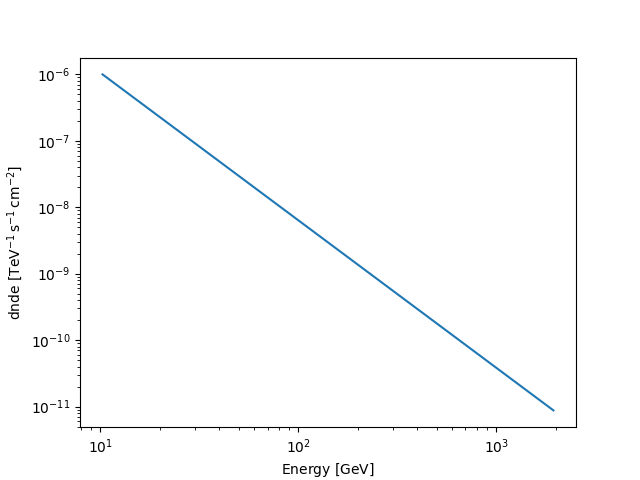
We assign the return axes object to variable called ax_crab_3fhl,
because we will reuse it later to plot the flux points on top.
To compute the differential flux at 100 GeV we can simply call the model like normal Python function and convert to the desired units:
print(crab_3fhl_spec(100 * u.GeV).to("cm-2 s-1 GeV-1"))
6.3848912826152664e-12 1 / (GeV s cm2)
Next we can compute the integral flux of the Crab between 10 GeV and 2000 GeV:
print(
    crab_3fhl_spec.integral(energy_min=10 * u.GeV, energy_max=2000 * u.GeV).to(
        "cm-2 s-1"
    )
)
8.67457342435522e-09 1 / (s cm2)
We can easily convince ourself, that it corresponds to the value given in the Fermi-LAT 3FHL catalog:
print(crab_3fhl.data["Flux"])
8.658909145253801e-09 1 / (s cm2)
In addition we can compute the energy flux between 10 GeV and 2000 GeV:
print(
    crab_3fhl_spec.energy_flux(energy_min=10 * u.GeV, energy_max=2000 * u.GeV).to(
        "erg cm-2 s-1"
    )
)
5.311489174710791e-10 erg / (s cm2)
Next we will access the flux points data of the Crab:
print(crab_3fhl.flux_points)
FluxPoints
----------

  geom                   : RegionGeom
  axes                   : ['lon', 'lat', 'energy']
  shape                  : (1, 1, 5)
  quantities             : ['norm', 'norm_errp', 'norm_errn', 'norm_ul', 'sqrt_ts', 'is_ul']
  ref. model             : pl
  n_sigma                : 1
  n_sigma_ul             : 2
  sqrt_ts_threshold_ul   : 1
  sed type init          : flux
If you want to learn more about the different flux point formats you can read the specification here.
No we can check again the underlying astropy data structure by accessing
the .table attribute:
print(crab_3fhl.flux_points.to_table(sed_type="dnde", formatted=True))
 e_ref    e_min   e_max         dnde      ...     dnde_ul     sqrt_ts is_ul
  GeV      GeV     GeV    1 / (TeV s cm2) ... 1 / (TeV s cm2)
-------- ------- -------- --------------- ... --------------- ------- -----
  14.142  10.000   20.000       5.120e-07 ...             nan 125.157 False
  31.623  20.000   50.000       7.359e-08 ...             nan  88.715 False
  86.603  50.000  150.000       9.024e-09 ...             nan  59.087 False
 273.861 150.000  500.000       7.660e-10 ...             nan  33.076 False
1000.000 500.000 2000.000       4.291e-11 ...             nan  15.573 False
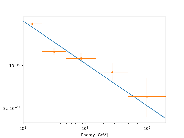
Finally let’s combine spectral model and flux points in a single plot
and scale with energy_power=2 to obtain the spectral energy
distribution:
/home/runner/work/gammapy-docs/gammapy-docs/gammapy/.tox/build_docs/lib/python3.12/site-packages/gammapy/maps/region/ndmap.py:154: UserWarning: This axis already has a converter set and is updating to a potentially incompatible converter
  ax.errorbar(
Exercises#
Plot the spectral model and flux points for PKS 2155-304 for the 3FGL and 2FHL catalogs. Try to plot the error of the model (aka “Butterfly”) as well.
What next?#
This was a quick introduction to some of the high level classes in Astropy and Gammapy.
To learn more about those classes, go to the API docs (links are in the introduction at the top).
To learn more about other parts of Gammapy (e.g. Fermi-LAT and TeV data analysis), check out the other tutorial notebooks.
To see what’s available in Gammapy, browse the Gammapy docs or use the full-text search.
If you have any questions, ask on the mailing list.