Note

Go to the end to download the full example code. or to run this example in your browser via Binder

Time resolved spectroscopy estimator#

Perform spectral fits of a blazar in different time bins to investigate spectral changes during flares.

Context#

The LightCurveEstimator in Gammapy (see light curve notebook, and light curve for flares notebook.) fits the amplitude in each time/energy bin, keeping the spectral shape frozen. However, in the analysis of flaring sources, it is often interesting to study not only how the flux changes with time but how the spectral shape varies with time.

Proposed approach#

The main idea behind doing a time resolved spectroscopy is to

Select relevant Observations from the DataStore
Define time intervals in which to fit the spectral model
Apply the above time selections on the data to obtain new Observations
Perform standard data reduction on the above data
Define a source model
Fit the reduced data in each time bin with the source model
Extract relevant information in a table

Here, we will use the PKS 2155-304 observations from the H.E.S.S. first public test data release.

We use time intervals of 15 minutes duration to explore spectral variability.

Setup#

As usual, we’ll start with some general imports…

import logging
import numpy as np
import astropy.units as u
from astropy.coordinates import Angle, SkyCoord
from astropy.table import QTable
from astropy.time import Time
from regions import CircleSkyRegion

# %matplotlib inline
import matplotlib.pyplot as plt

log = logging.getLogger(__name__)

from gammapy.data import DataStore
from gammapy.datasets import Datasets, SpectrumDataset
from gammapy.makers import (
    ReflectedRegionsBackgroundMaker,
    SafeMaskMaker,
    SpectrumDatasetMaker,
)
from gammapy.maps import MapAxis, RegionGeom, TimeMapAxis
from gammapy.modeling import Fit
from gammapy.modeling.models import (
    PowerLawSpectralModel,
    SkyModel,
)

log = logging.getLogger(__name__)

Data selection#

We select all runs pointing within 2 degrees of PKS 2155-304.

data_store = DataStore.from_dir("$GAMMAPY_DATA/hess-dl3-dr1/")
target_position = SkyCoord(329.71693826 * u.deg, -30.2255890 * u.deg, frame="icrs")
selection = dict(
    type="sky_circle",
    frame="icrs",
    lon=target_position.ra,
    lat=target_position.dec,
    radius=2 * u.deg,
)
obs_ids = data_store.obs_table.select_observations(selection)["OBS_ID"]
observations = data_store.get_observations(obs_ids)
print(f"Number of selected observations : {len(observations)}")

Number of selected observations : 21

The flaring observations were taken during July 2006. We define 15-minute time intervals as lists of Time start and stop objects, and apply the intervals to the observations by using select_time

t0 = Time("2006-07-29T20:30")
duration = 15 * u.min
n_time_bins = 25
times = t0 + np.arange(n_time_bins) * duration

time_intervals = [Time([tstart, tstop]) for tstart, tstop in zip(times[:-1], times[1:])]
print(time_intervals[-1].mjd)
short_observations = observations.select_time(time_intervals)

# check that observations have been filtered
print(f"Number of observations after time filtering: {len(short_observations)}\n")
print(short_observations[1].gti)

[53946.09375    53946.10416667]
Number of observations after time filtering: 34

GTI info:
- Number of GTIs: 1
- Duration: 461.99999999999545 s
- Start: 207521165.184 s MET
- Start: 2006-07-29T20:45:00.000 (time standard: UTC)
- Stop: 207521627.184 s MET
- Stop: 2006-07-29T20:53:47.184 (time standard: TT)

Data reduction#

In this example, we perform a 1D analysis with a reflected regions background estimation. For details, see the Spectral analysis tutorial.

energy_axis = MapAxis.from_energy_bounds("0.4 TeV", "20 TeV", nbin=10)
energy_axis_true = MapAxis.from_energy_bounds(
    "0.1 TeV", "40 TeV", nbin=20, name="energy_true"
)

on_region_radius = Angle("0.11 deg")
on_region = CircleSkyRegion(center=target_position, radius=on_region_radius)

geom = RegionGeom.create(region=on_region, axes=[energy_axis])

dataset_maker = SpectrumDatasetMaker(
    containment_correction=True, selection=["counts", "exposure", "edisp"]
)
bkg_maker = ReflectedRegionsBackgroundMaker()
safe_mask_masker = SafeMaskMaker(methods=["aeff-max"], aeff_percent=10)

datasets = Datasets()

dataset_empty = SpectrumDataset.create(geom=geom, energy_axis_true=energy_axis_true)

for obs in short_observations:
    dataset = dataset_maker.run(dataset_empty.copy(), obs)

    dataset_on_off = bkg_maker.run(dataset, obs)
    dataset_on_off = safe_mask_masker.run(dataset_on_off, obs)
    datasets.append(dataset_on_off)

This gives us list of SpectrumDatasetOnOff which can now be modelled.

print(datasets)

Datasets
--------

Dataset 0:

  Type       : SpectrumDatasetOnOff
  Name       : 95dsGeon
  Instrument : HESS
  Models     :

Dataset 1:

  Type       : SpectrumDatasetOnOff
  Name       : 2n4dDaJq
  Instrument : HESS
  Models     :

Dataset 2:

  Type       : SpectrumDatasetOnOff
  Name       : eaNCHpPQ
  Instrument : HESS
  Models     :

Dataset 3:

  Type       : SpectrumDatasetOnOff
  Name       : QCbYj3hq
  Instrument : HESS
  Models     :

Dataset 4:

  Type       : SpectrumDatasetOnOff
  Name       : L0SVc1er
  Instrument : HESS
  Models     :

Dataset 5:

  Type       : SpectrumDatasetOnOff
  Name       : nZvz1Xlp
  Instrument : HESS
  Models     :

Dataset 6:

  Type       : SpectrumDatasetOnOff
  Name       : I9KyEo3q
  Instrument : HESS
  Models     :

Dataset 7:

  Type       : SpectrumDatasetOnOff
  Name       : 7tEO75Ft
  Instrument : HESS
  Models     :

Dataset 8:

  Type       : SpectrumDatasetOnOff
  Name       : 5W-AgQ4g
  Instrument : HESS
  Models     :

Dataset 9:

  Type       : SpectrumDatasetOnOff
  Name       : mJUabcEI
  Instrument : HESS
  Models     :

Dataset 10:

  Type       : SpectrumDatasetOnOff
  Name       : P-KETQb4
  Instrument : HESS
  Models     :

Dataset 11:

  Type       : SpectrumDatasetOnOff
  Name       : DiTZHzUj
  Instrument : HESS
  Models     :

Dataset 12:

  Type       : SpectrumDatasetOnOff
  Name       : BebvcYC-
  Instrument : HESS
  Models     :

Dataset 13:

  Type       : SpectrumDatasetOnOff
  Name       : 9UkDz0S4
  Instrument : HESS
  Models     :

Dataset 14:

  Type       : SpectrumDatasetOnOff
  Name       : V8JPq_8b
  Instrument : HESS
  Models     :

Dataset 15:

  Type       : SpectrumDatasetOnOff
  Name       : parw31fx
  Instrument : HESS
  Models     :

Dataset 16:

  Type       : SpectrumDatasetOnOff
  Name       : yBNaNxAC
  Instrument : HESS
  Models     :

Dataset 17:

  Type       : SpectrumDatasetOnOff
  Name       : V7EYczzf
  Instrument : HESS
  Models     :

Dataset 18:

  Type       : SpectrumDatasetOnOff
  Name       : 4heaD3c0
  Instrument : HESS
  Models     :

Dataset 19:

  Type       : SpectrumDatasetOnOff
  Name       : VLQ_IgMJ
  Instrument : HESS
  Models     :

Dataset 20:

  Type       : SpectrumDatasetOnOff
  Name       : hVOkaMde
  Instrument : HESS
  Models     :

Dataset 21:

  Type       : SpectrumDatasetOnOff
  Name       : YfR3-UlV
  Instrument : HESS
  Models     :

Dataset 22:

  Type       : SpectrumDatasetOnOff
  Name       : uUzKMrbK
  Instrument : HESS
  Models     :

Dataset 23:

  Type       : SpectrumDatasetOnOff
  Name       : jWaiR6Fg
  Instrument : HESS
  Models     :

Dataset 24:

  Type       : SpectrumDatasetOnOff
  Name       : QQla_yO8
  Instrument : HESS
  Models     :

Dataset 25:

  Type       : SpectrumDatasetOnOff
  Name       : FUl4aSPg
  Instrument : HESS
  Models     :

Dataset 26:

  Type       : SpectrumDatasetOnOff
  Name       : jDW4nSdc
  Instrument : HESS
  Models     :

Dataset 27:

  Type       : SpectrumDatasetOnOff
  Name       : AVGia3EG
  Instrument : HESS
  Models     :

Dataset 28:

  Type       : SpectrumDatasetOnOff
  Name       : Xh556Ys4
  Instrument : HESS
  Models     :

Dataset 29:

  Type       : SpectrumDatasetOnOff
  Name       : lZao3SGN
  Instrument : HESS
  Models     :

Dataset 30:

  Type       : SpectrumDatasetOnOff
  Name       : ys6CV6Dd
  Instrument : HESS
  Models     :

Dataset 31:

  Type       : SpectrumDatasetOnOff
  Name       : ZqxzxScH
  Instrument : HESS
  Models     :

Dataset 32:

  Type       : SpectrumDatasetOnOff
  Name       : QRSMZ-L3
  Instrument : HESS
  Models     :

Dataset 33:

  Type       : SpectrumDatasetOnOff
  Name       : 3GiZg14_
  Instrument : HESS
  Models     :

Modeling#

We will first fit a simple power law model in each time bin. Note that since we are using an on-off analysis here, no background model is required. If you are doing a 3D FoV analysis, you will need to model the background appropriately as well.

The index and amplitude of the spectral model is kept free. You can configure the quantities you want to freeze.

spectral_model = PowerLawSpectralModel(
    index=3.0, amplitude=2e-11 * u.Unit("1 / (cm2 s TeV)"), reference=1 * u.TeV
)
spectral_model.parameters["index"].frozen = False


sky_model = SkyModel(spatial_model=None, spectral_model=spectral_model, name="pks2155")
print(sky_model)

SkyModel

  Name                      : pks2155
  Datasets names            : None
  Spectral model type       : PowerLawSpectralModel
  Spatial  model type       :
  Temporal model type       :
  Parameters:
    index                         :      3.000   +/-    0.00
    amplitude                     :   2.00e-11   +/- 0.0e+00 1 / (TeV s cm2)
    reference             (frozen):      1.000       TeV

Time resolved spectroscopy algorithm#

The following function is the crux of this tutorial. The sky_model is fit in each bin and a list of fit_results stores the fit information in each bin.

If time bins are present without any available observations, those bins are discarded and a new list of valid time intervals and fit results are created.

def time_resolved_spectroscopy(datasets, model, time_intervals):
    fit = Fit()
    valid_intervals = []
    fit_results = []
    index = 0
    for t_min, t_max in time_intervals:
        datasets_to_fit = datasets.select_time(time_min=t_min, time_max=t_max)

        if len(datasets_to_fit) == 0:
            log.info(
                f"No Dataset for the time interval {t_min} to {t_max}. Skipping interval."
            )
            continue

        model_in_bin = model.copy(name="Model_bin_" + str(index))
        datasets_to_fit.models = model_in_bin
        result = fit.run(datasets_to_fit)
        fit_results.append(result)
        valid_intervals.append([t_min, t_max])
        index += 1

    return valid_intervals, fit_results

We now apply it to our data

valid_times, results = time_resolved_spectroscopy(datasets, sky_model, time_intervals)

/home/runner/work/gammapy-docs/gammapy-docs/gammapy/.tox/build_docs/lib/python3.9/site-packages/numpy/core/fromnumeric.py:88: RuntimeWarning: overflow encountered in reduce
  return ufunc.reduce(obj, axis, dtype, out, **passkwargs)
/home/runner/work/gammapy-docs/gammapy-docs/gammapy/.tox/build_docs/lib/python3.9/site-packages/numpy/core/fromnumeric.py:88: RuntimeWarning: overflow encountered in reduce
  return ufunc.reduce(obj, axis, dtype, out, **passkwargs)

To view the results of the fit,

print(results[0])

OptimizeResult

        backend    : minuit
        method     : migrad
        success    : True
        message    : Optimization terminated successfully.
        nfev       : 76
        total stat : 6.00

CovarianceResult

        backend    : minuit
        method     : hesse
        success    : True
        message    : Hesse terminated successfully.

Or, to access the fitted models,

print(results[0].models)

DatasetModels

Component 0: SkyModel

  Name                      : Model_bin_0
  Datasets names            : None
  Spectral model type       : PowerLawSpectralModel
  Spatial  model type       :
  Temporal model type       :
  Parameters:
    index                         :      4.009   +/-    0.35
    amplitude                     :   1.02e-10   +/- 1.3e-11 1 / (TeV s cm2)
    reference             (frozen):      1.000       TeV

To better visualise the data, we can create a table by extracting some relevant information. In the following, we extract the time intervals, information on the fit convergence and the free parameters. You can extract more information if required, eg, the total_stat in each bin, etc.

def create_table(time_intervals, fit_result):
    t = QTable()

    t["tstart"] = np.array(time_intervals).T[0]
    t["tstop"] = np.array(time_intervals).T[1]
    t["convergence"] = [result.success for result in fit_result]
    for par in fit_result[0].models.parameters.free_parameters:
        t[par.name] = [
            result.models.parameters[par.name].value * par.unit for result in fit_result
        ]
        t[par.name + "_err"] = [
            result.models.parameters[par.name].error * par.unit for result in fit_result
        ]

    return t


table = create_table(valid_times, results)
print(table)

         tstart                  tstop          ...     amplitude_err
                                                ...    1 / (TeV s cm2)
----------------------- ----------------------- ... ----------------------
2006-07-29T20:30:00.000 2006-07-29T20:45:00.000 ... 1.2923272203680937e-11
2006-07-29T20:45:00.000 2006-07-29T21:00:00.000 ... 1.1393881668086242e-11
2006-07-29T21:00:00.000 2006-07-29T21:15:00.000 ...  9.820734654694367e-12
2006-07-29T21:15:00.000 2006-07-29T21:30:00.000 ...   1.00336861061002e-11
2006-07-29T21:30:00.000 2006-07-29T21:45:00.000 ... 1.0859117235629056e-11
2006-07-29T21:45:00.000 2006-07-29T22:00:00.000 ... 1.1661916367760008e-11
2006-07-29T22:00:00.000 2006-07-29T22:15:00.000 ...  9.683535101178161e-12
2006-07-29T22:15:00.000 2006-07-29T22:30:00.000 ...   9.20016447648031e-12
2006-07-29T22:30:00.000 2006-07-29T22:45:00.000 ...  8.243742672227972e-12
2006-07-29T22:45:00.000 2006-07-29T23:00:00.000 ...   8.68588096384626e-12
                    ...                     ... ...                    ...
2006-07-30T00:00:00.000 2006-07-30T00:15:00.000 ...   8.53849342472254e-12
2006-07-30T00:15:00.000 2006-07-30T00:30:00.000 ...  5.597194451442478e-12
2006-07-30T00:30:00.000 2006-07-30T00:45:00.000 ...  6.166871893629602e-12
2006-07-30T00:45:00.000 2006-07-30T01:00:00.000 ...  5.871730083414263e-12
2006-07-30T01:00:00.000 2006-07-30T01:15:00.000 ... 6.9721952295357764e-12
2006-07-30T01:15:00.000 2006-07-30T01:30:00.000 ...  6.373892759762174e-12
2006-07-30T01:30:00.000 2006-07-30T01:45:00.000 ...  6.397035933646679e-12
2006-07-30T01:45:00.000 2006-07-30T02:00:00.000 ...  5.282951078740491e-12
2006-07-30T02:00:00.000 2006-07-30T02:15:00.000 ... 5.7115414505410296e-12
2006-07-30T02:15:00.000 2006-07-30T02:30:00.000 ...  4.579178801616083e-12
Length = 24 rows

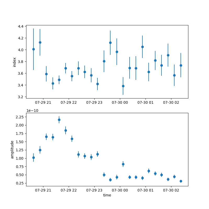
Visualising the results#

We can plot the spectral index and the amplitude as a function of time. For convenience, we will convert the times into a TimeMapAxis.

time_axis = TimeMapAxis.from_time_edges(
    time_min=table["tstart"], time_max=table["tstop"]
)

fix, axes = plt.subplots(2, 1, figsize=(8, 8))
axes[0].errorbar(
    x=time_axis.as_plot_center, y=table["index"], yerr=table["index_err"], fmt="o"
)
axes[1].errorbar(
    x=time_axis.as_plot_center,
    y=table["amplitude"],
    yerr=table["amplitude_err"],
    fmt="o",
)

axes[0].set_ylabel("index")
axes[1].set_ylabel("amplitude")
axes[1].set_xlabel("time")
plt.show()

To get the integrated flux, we can access the model stored in the fit result object, eg

integral_flux = (
    results[0]
    .models[0]
    .spectral_model.integral_error(energy_min=1 * u.TeV, energy_max=10 * u.TeV)
)
print("Integral flux in the first bin:", integral_flux)

Integral flux in the first bin: [3.39200283e-11 4.59497703e-12] 1 / (s cm2)

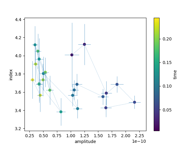
To plot hysteresis curves, ie the spectral index as a function of amplitude

plt.errorbar(
    table["amplitude"],
    table["index"],
    xerr=table["amplitude_err"],
    yerr=table["index_err"],
    linestyle=":",
    linewidth=0.5,
)
plt.scatter(table["amplitude"], table["index"], c=time_axis.center.value)
plt.xlabel("amplitude")
plt.ylabel("index")
plt.colorbar().set_label("time")
plt.show()

Exercises#

Quantify the variability in the spectral index
Rerun the algorithm using a different spectral shape, such as a broken power law.
Compare the significance of the new model with the simple power law. Take note of any fit non-convergence in the bins.

Total running time of the script: (0 minutes 22.198 seconds)

Gallery generated by Sphinx-Gallery