Note
Go to the end to download the full example code or to run this example in your browser via Binder.
MAGIC with Gammapy#
Explore the MAGIC IRFs and perform a point like spectral analysis with energy dependent offset cut.
Introduction#
MAGIC (Major Atmospheric Gamma Imaging
Cherenkov Telescopes) consists of two Imaging Atmospheric Cherenkov telescopes in La Palma, Spain.
These 17m diameter telescopes detect gamma-rays from ~ 30 GeV to 100 TeV.
The MAGIC public data release contains around 100 hours of data and can be found here.
This notebook presents an analysis based on just two runs of the Crab Nebula.
It provides an introduction to using the MAGIC DL3 data products, to produce a
SpectrumDatasetOnOff. Importantly it shows how to perform a data reduction
with energy-dependent directional cuts, as described further below.
For further information, see this paper.
Prerequisites#
Understanding the basic data reduction performed in the Spectral analysis tutorial.
understanding the difference between a point-like and a full-enclosure IRF.
Context#
As described in the Spectral analysis tutorial, the background is estimated from the field of view (FoV) of the observation. Since the MAGIC data release does not include a dedicated background IRF, this estimation must be performed directly from the FoV. In particular, the source and background events are counted within a circular ON region enclosing the source. The background to be subtracted is then estimated from one or more OFF regions with an expected background rate similar to the one in the ON region (i.e. from regions with similar acceptance).
Full-containment IRFs have no directional cut applied, when employed for a 1D analysis, it is required to apply a correction to the IRF accounting for flux leaking out of the ON region. This correction is typically obtained by integrating the PSF within the ON region.
When computing a point-like IRFs, a directional cut around the assumed source position is applied to the simulated events. For this IRF type, no PSF component is provided. The size of the ON and OFF regions used for the spectrum extraction should then reflect this cut, since a response computed within a specific region around the source is being provided.
The directional cut is typically an angular distance from the assumed source position, \(\theta\). The gamma-astro-data-format specifications offer two different ways to store this information:
if the same \(\theta\) cut is applied at all energies and offsets, a RAD_MAX keyword is added to the header of the data units containing IRF components. This should be used to define the size of the ON and OFF regions;
in case an energy-dependent (and offset-dependent) \(\theta\) cut is applied, its values are stored in additional
FITSdata unit, named RAD_MAX_2D.
Gammapy provides a class to automatically read these values,
RadMax2D, for both cases (fixed or energy-dependent
\(\theta\) cut). In this notebook we will focus on how to perform a
spectral extraction with a point-like IRF with an energy-dependent
\(\theta\) cut. We remark that in this case a
PointSkyRegion (and not a CircleSkyRegion)
should be used to define the ON region. If a geometry based on a
PointSkyRegion is fed to the spectra and the background
Maker, the latter will automatically use the values stored in the
RAD_MAX keyword / table for defining the size of the ON and OFF
regions.
Beside the definition of the ON region during the data reduction, the remaining steps are identical to the other Spectral analysis tutorial, so we will not detail the data reduction steps already presented in the other tutorial.
Objective: perform the data reduction and analysis of 2 Crab Nebula observations of MAGIC and fit the resulting datasets.
Setup#
As usual, we’ll start with some setup …
from IPython.display import display
import astropy.units as u
from astropy.coordinates import SkyCoord
from regions import PointSkyRegion

# %matplotlib inline
import matplotlib.pyplot as plt

from gammapy.data import DataStore
from gammapy.datasets import Datasets, SpectrumDataset
from gammapy.makers import (
    ReflectedRegionsBackgroundMaker,
    SafeMaskMaker,
    SpectrumDatasetMaker,
    WobbleRegionsFinder,
)
from gammapy.maps import Map, MapAxis, RegionGeom
from gammapy.modeling import Fit
from gammapy.modeling.models import (
    LogParabolaSpectralModel,
    SkyModel,
    create_crab_spectral_model,
)
from gammapy.visualization import plot_spectrum_datasets_off_regions
Load data#
We load the two MAGIC observations of the Crab Nebula which contain a
RAD_MAX_2D table.
data_store = DataStore.from_dir("$GAMMAPY_DATA/magic/rad_max/data")
observations = data_store.get_observations(required_irf="point-like")
We can take a look at the MAGIC IRFs:
observations[0].peek()
plt.show()
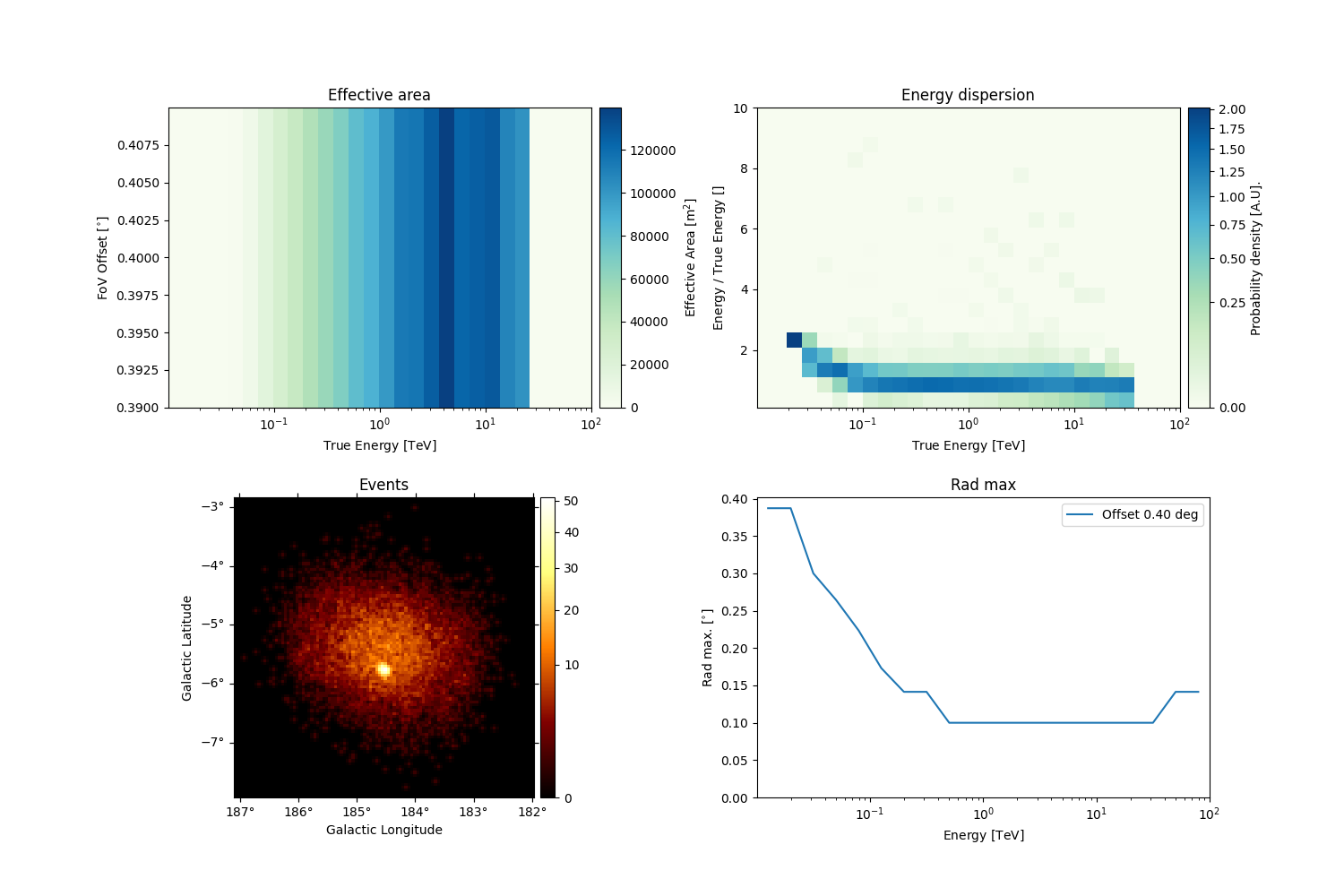
The rad_max attribute, containing the RAD_MAX_2D table, is
automatically loaded in the observation. As we can see from the IRF
component axes, the table has a single offset value and 28 estimated
energy values.
rad_max = observations["5029747"].rad_max
print(rad_max)
RadMax2D
--------

  axes  : ['energy', 'offset']
  shape : (20, 1)
  ndim  : 2
  unit  : deg
  dtype : >f4
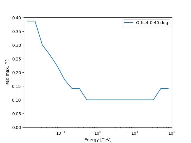
Plotting the rad max value against the energy:
Define the ON region#
To use the RAD_MAX_2D values to define the sizes of the ON and OFF
regions it is necessary to specify the ON region as
a PointSkyRegion i.e. we specify only the center of our ON region.
target_position = SkyCoord(ra=83.63, dec=22.01, unit="deg", frame="icrs")
on_region = PointSkyRegion(target_position)
Run data reduction chain#
We begin by configuring the dataset maker classes. First, we define the reconstructed and true energy axes:
energy_axis = MapAxis.from_energy_bounds(
    50, 1e5, nbin=5, per_decade=True, unit="GeV", name="energy"
)
energy_axis_true = MapAxis.from_energy_bounds(
    10, 1e5, nbin=10, per_decade=True, unit="GeV", name="energy_true"
)
We create a RegionGeom by combining the ON region with the
estimated energy axis of the SpectrumDataset we want to produce.
This geometry in used to create the SpectrumDataset.
geom = RegionGeom.create(region=on_region, axes=[energy_axis])

dataset_empty = SpectrumDataset.create(geom=geom, energy_axis_true=energy_axis_true)
The SpectrumDatasetMaker and ReflectedRegionsBackgroundMaker
will utilise the \(\theta\) values in rad_max to define
the sizes of the OFF regions.
dataset_maker = SpectrumDatasetMaker(
    containment_correction=False, selection=["counts", "exposure", "edisp"]
)
In order to define the OFF regions it is recommended to use a
WobbleRegionsFinder, that uses fixed positions for
the OFF regions. In the different estimated energy bins we will have OFF
regions centered at the same positions, but with changing size.
The parameter n_off_regions specifies the number of OFF regions to be considered.
In this case we use 3.
region_finder = WobbleRegionsFinder(n_off_regions=3)
bkg_maker = ReflectedRegionsBackgroundMaker(region_finder=region_finder)
Use the energy threshold specified in the DL3 files for the safe mask:
safe_mask_masker = SafeMaskMaker(methods=["aeff-default"])

datasets = Datasets()
Create a counts map for visualisation later:
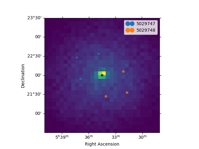
counts = Map.create(skydir=target_position, width=3)
Perform the data reduction loop:
for observation in observations:
    dataset = dataset_maker.run(
        dataset_empty.copy(name=str(observation.obs_id)), observation
    )
    counts.fill_events(observation.events)
    dataset_on_off = bkg_maker.run(dataset, observation)
    dataset_on_off = safe_mask_masker.run(dataset_on_off, observation)
    datasets.append(dataset_on_off)
Now we can plot the off regions and target positions on top of the counts map:
ax = counts.plot(cmap="viridis")
geom.plot_region(ax=ax, kwargs_point={"color": "k", "marker": "*"})
plot_spectrum_datasets_off_regions(ax=ax, datasets=datasets)
plt.show()
Fit spectrum#
We perform a joint likelihood fit of the two datasets. For this particular datasets we select a fit range between \(80\,{\rm GeV}\) and \(20\,{\rm TeV}\).
e_min = 80 * u.GeV
e_max = 20 * u.TeV

for dataset in datasets:
    dataset.mask_fit = dataset.counts.geom.energy_mask(e_min, e_max)

spectral_model = LogParabolaSpectralModel(
    amplitude=1e-12 * u.Unit("cm-2 s-1 TeV-1"),
    alpha=2,
    beta=0.1,
    reference=1 * u.TeV,
)
model = SkyModel(spectral_model=spectral_model, name="crab")

datasets.models = [model]

fit = Fit()
result = fit.run(datasets=datasets)

# we make a copy here to compare it later
best_fit_model = model.copy()
/home/runner/work/gammapy-docs/gammapy-docs/gammapy/.tox/build_docs/lib/python3.12/site-packages/numpy/_core/fromnumeric.py:83: RuntimeWarning: overflow encountered in reduce
  return ufunc.reduce(obj, axis, dtype, out, **passkwargs)
Fit quality and model residuals#
We can access the results dictionary to see if the fit converged:
print(result)
OptimizeResult

        backend    : minuit
        method     : migrad
        success    : True
        message    : Optimization terminated successfully.
        nfev       : 213
        total stat : 23.98

CovarianceResult

        backend    : minuit
        method     : hesse
        success    : True
        message    : Hesse terminated successfully.
and check the best-fit parameters
display(datasets.models.to_parameters_table())
model type    name     value         unit      ... min max frozen link prior
----- ---- --------- ---------- -------------- ... --- --- ------ ---- -----
 crab      amplitude 4.2903e-11 TeV-1 s-1 cm-2 ... nan nan  False
 crab      reference 1.0000e+00            TeV ... nan nan   True
 crab          alpha 2.5819e+00                ... nan nan  False
 crab           beta 1.9580e-01                ... nan nan  False
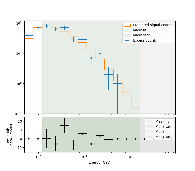
A simple way to inspect the model residuals is using the function
plot_fit()
ax_spectrum, ax_residuals = datasets[0].plot_fit()
ax_spectrum.set_ylim(0.1, 120)
plt.show()
For more ways of assessing fit quality, please refer to the dedicated Fitting tutorial.
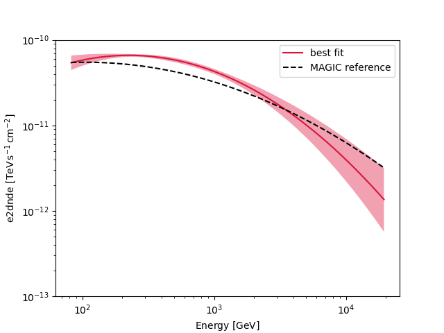
Compare against the literature#
Let us compare the spectrum we obtained against a previous measurement by MAGIC.
fig, ax = plt.subplots()
plot_kwargs = {
    "energy_bounds": [0.08, 20] * u.TeV,
    "sed_type": "e2dnde",
    "ax": ax,
}
ax.yaxis.set_units(u.Unit("TeV cm-2 s-1"))
ax.xaxis.set_units(u.Unit("GeV"))
crab_magic_lp = create_crab_spectral_model("magic_lp")

best_fit_model.spectral_model.plot(
    ls="-", lw=1.5, color="crimson", label="best fit", **plot_kwargs
)
best_fit_model.spectral_model.plot_error(facecolor="crimson", alpha=0.4, **plot_kwargs)
crab_magic_lp.plot(ls="--", lw=1.5, color="k", label="MAGIC reference", **plot_kwargs)

ax.legend()
ax.set_ylim([1e-13, 1e-10])
plt.show()
/home/runner/work/gammapy-docs/gammapy-docs/gammapy/.tox/build_docs/lib/python3.12/site-packages/gammapy/modeling/models/spectral.py:649: UserWarning: This axis already has a converter set and is updating to a potentially incompatible converter
  ax.plot(energy.center, flux.quantity[:, 0, 0], **kwargs)
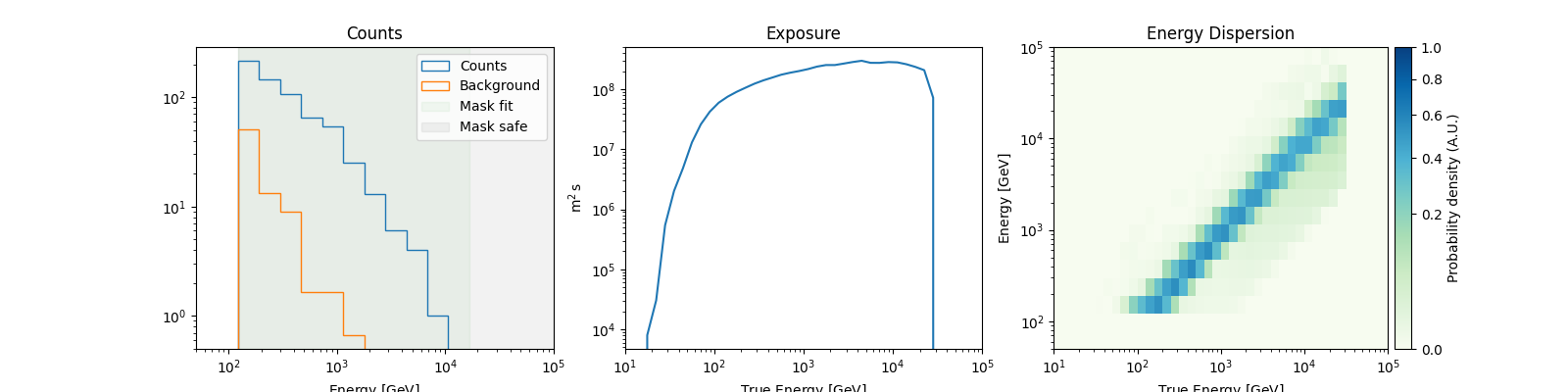
Dataset simulations#
A common way to check if a fit is biased is to simulate multiple datasets with the obtained best fit model, and check the distribution of the fitted parameters. Here, we show how to perform one such simulation assuming the measured off counts provide a good distribution of the background.
dataset_simulated = datasets.stack_reduce().copy(name="simulated_ds")
simulated_model = best_fit_model.copy(name="simulated")
dataset_simulated.models = simulated_model
dataset_simulated.fake(
    npred_background=dataset_simulated.counts_off * dataset_simulated.alpha
)
dataset_simulated.peek()
plt.show()
/home/runner/work/gammapy-docs/gammapy-docs/gammapy/.tox/build_docs/lib/python3.12/site-packages/gammapy/maps/core.py:1918: RuntimeWarning: invalid value encountered in divide
  out.data = operator(out.data, other_data)
The important thing to note here is that while this samples the on-counts, the off counts are not sampled. If you have multiple measurements of the off counts, they should be used. Alternatively, you can try to create a parametric model of the background.
result = fit.run(datasets=[dataset_simulated])
print(result.models.to_parameters_table())
  model   type    name     value         unit      ... min max frozen link prior
--------- ---- --------- ---------- -------------- ... --- --- ------ ---- -----
simulated      amplitude 3.7863e-11 TeV-1 s-1 cm-2 ... nan nan  False
simulated      reference 1.0000e+00            TeV ... nan nan   True
simulated          alpha 2.5048e+00                ... nan nan  False
simulated           beta 1.1011e-01                ... nan nan  False