HAWC with Gammapy

Explore HAWC event lists and instrument response functions (IRFs), then perform the data reduction steps.

Introduction

HAWC is an array of water Cherenkov detectors located in Mexico that detects gamma-rays in the range between hundreds of GeV and hundreds of TeV. Gammapy recently added support of HAWC high level data analysis, after export to the current open data level 3 format.

The HAWC data is largely private. However, in 2022, a small sub-set of HAWC Pass4 event lists from the Crab nebula region was publicly released. This dataset is 1 GB in size, so only a subset will be used here as an example.

Tutorial overview

This notebook is a quick introduction to HAWC data analysis with Gammapy. It briefly describes the HAWC data and how to access it, and then uses a subset of the data to produce a MapDataset, to show how the data reduction is performed.

The HAWC data release contains events where the energy is estimated using two different algorithms, referred to as “NN” and “GP” (see this paper for a detailed description). These two event classes are not independent, meaning that events are repeated between the NN and GP datasets. Therefore, these data should never be analysed jointly, and one of the two estimators needs to be chosen before proceeding.

Once the data has been reduced to a MapDataset, there are no differences in the way that HAWC data is handled with respect to data from any other observatory, such as H.E.S.S. or CTAO.

HAWC data access and reduction

This is how to access data and IRFs from the HAWC Crab event data release.

import astropy.units as u
from astropy.coordinates import SkyCoord
import matplotlib.pyplot as plt
from gammapy.data import DataStore, HDUIndexTable, ObservationTable
from gammapy.datasets import MapDataset
from gammapy.estimators import ExcessMapEstimator
from gammapy.makers import MapDatasetMaker, SafeMaskMaker
from gammapy.maps import Map, MapAxis, WcsGeom

Check setup

from gammapy.utils.check import check_tutorials_setup

check_tutorials_setup()

System:

        python_executable      : /home/runner/work/gammapy-docs/gammapy-docs/gammapy/.tox/build_docs/bin/python
        python_version         : 3.9.20
        machine                : x86_64
        system                 : Linux


Gammapy package:

        version                : 2.0.dev2+g10bce85c9
        path                   : /home/runner/work/gammapy-docs/gammapy-docs/gammapy/.tox/build_docs/lib/python3.9/site-packages/gammapy


Other packages:

        numpy                  : 1.26.4
        scipy                  : 1.13.1
        astropy                : 5.2.2
        regions                : 0.8
        click                  : 8.1.7
        yaml                   : 6.0.2
        IPython                : 8.18.1
        jupyterlab             : not installed
        matplotlib             : 3.9.2
        pandas                 : not installed
        healpy                 : 1.17.3
        iminuit                : 2.30.1
        sherpa                 : 4.16.1
        naima                  : 0.10.0
        emcee                  : 3.1.6
        corner                 : 2.2.2
        ray                    : 2.38.0


Gammapy environment variables:

        GAMMAPY_DATA           : /home/runner/work/gammapy-docs/gammapy-docs/gammapy-datasets/dev

Chose which estimator we will use

energy_estimator = "NN"

A useful way to organize the relevant files are with index tables. The observation index table contains information on each particular observation, such as the run ID. The HDU index table has a row per relevant file (i.e., events, effective area, psf…) and contains the path to said file. The HAWC data is divided into different event types, classified using the fraction of the array that was triggered by an event, a quantity usually referred to as “fHit”. These event types are fully independent, meaning that an event will have a unique event type identifier, which is usually a number indicating which fHit bin the event corresponds to. For this reason, a single HAWC observation has several HDU index tables associated to it, one per event type. In each table, there will be paths to a distinct event list file and IRFs. In the HAWC event data release, all the HDU tables are saved into the same FITS file, and can be accesses through the choice of the hdu index.

Load the tables

data_path = "$GAMMAPY_DATA/hawc/crab_events_pass4/"
hdu_filename = f"hdu-index-table-{energy_estimator}-Crab.fits.gz"
obs_filename = f"obs-index-table-{energy_estimator}-Crab.fits.gz"

There is only one observation table

obs_table = ObservationTable.read(data_path + obs_filename)

The remainder of this tutorial utilises just one fHit value, however, for a regular analysis you should combine all fHit bins. Here, we utilise fHit bin number 6. We start by reading the HDU index table of this fHit bin

fHit = 6
hdu_table = HDUIndexTable.read(data_path + hdu_filename, hdu=fHit)

From the tables, we can create a DataStore.

data_store = DataStore(hdu_table=hdu_table, obs_table=obs_table)

data_store.info()

Data store:
HDU index table:
BASE_DIR: /home/runner/work/gammapy-docs/gammapy-docs/gammapy-datasets/dev/hawc/crab_events_pass4
Rows: 6
OBS_ID: 103000133 -- 103000133
HDU_TYPE: ['aeff', 'bkg', 'edisp', 'events', 'gti', 'psf']
HDU_CLASS: ['edisp_kernel_map', 'events', 'gti', 'map', 'psf_map_reco']


Observation table:
Observatory name: 'N/A'
Number of observations: 1

There is only one observation

obs = data_store.get_observations()[0]

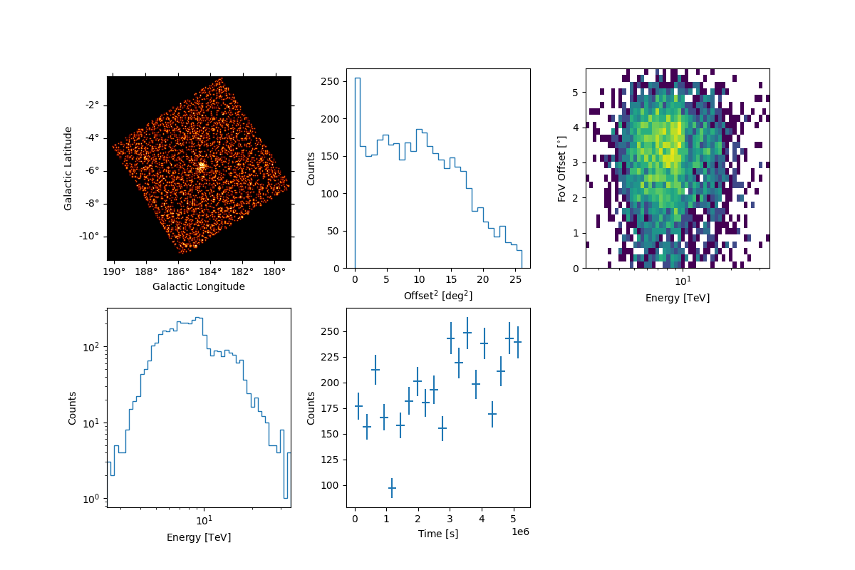
Peek events from this observation

obs.events.peek()
plt.show()

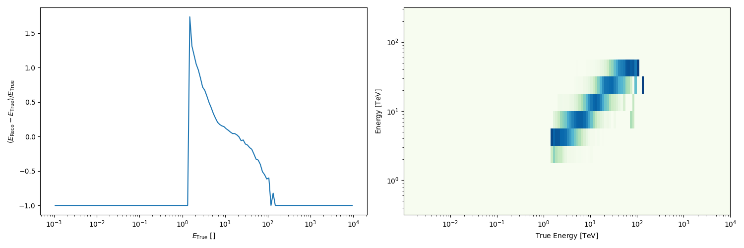
Peek the energy dispersion:

obs.edisp.peek()
plt.show()

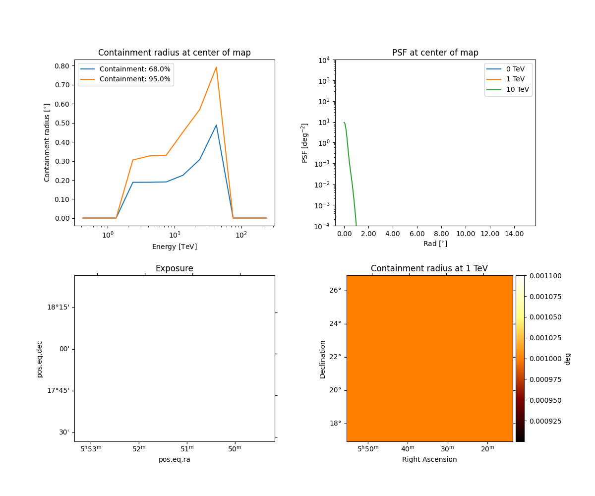
Peek the psf:

obs.psf.peek()
plt.show()

Peek the background for one transit:

plt.figure()
obs.bkg.reduce_over_axes().plot(add_cbar=True)
plt.show()

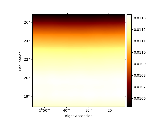
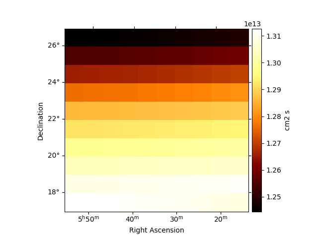
Peek the effective exposure for one transit:

plt.figure()
obs.aeff.reduce_over_axes().plot(add_cbar=True)
plt.show()

Data reduction into a MapDataset

We will now produce a MapDataset using the data from one of the fHit bins. In order to use all bins, one just needs to repeat this process inside a for loop that modifies the variable fHit.

First we define the geometry and axes, starting with the energy reco axis:

energy_axis = MapAxis.from_edges(
    [1.00, 1.78, 3.16, 5.62, 10.0, 17.8, 31.6, 56.2, 100, 177, 316] * u.TeV,
    name="energy",
    interp="log",
)

Note: this axis is the one used to create the background model map. If different edges are used, the MapDatasetMaker will interpolate between them, which might lead to unexpected behaviour.

Define the energy true axis:

energy_axis_true = MapAxis.from_energy_bounds(
    1e-3, 1e4, nbin=140, unit="TeV", name="energy_true"
)

Finally, create a geometry around the Crab location:

geom = WcsGeom.create(
    skydir=SkyCoord(ra=83.63, dec=22.01, unit="deg", frame="icrs"),
    width=6 * u.deg,
    axes=[energy_axis],
    binsz=0.05,
)

Define the makers we will use:

maker = MapDatasetMaker(selection=["counts", "background", "exposure", "edisp", "psf"])
safe_mask_maker = SafeMaskMaker(methods=["aeff-max"], aeff_percent=10)

Create an empty MapDataset. The keyword reco_psf=True is needed because the HAWC PSF is derived in reconstructed energy.

dataset_empty = MapDataset.create(
    geom, energy_axis_true=energy_axis_true, name=f"fHit {fHit}", reco_psf=True
)
dataset = maker.run(dataset_empty, obs)

The livetime information is used by the SafeMaskMaker to retrieve the effective area from the exposure. The HAWC effective area is computed for one source transit above 45º zenith, which is around 6h. Since the effective area condition used here is relative to the maximum, this value does not actually impact the result.

dataset.exposure.meta["livetime"] = "6 h"
dataset = safe_mask_maker.run(dataset)

Now we have a dataset that has background and exposure quantities for one single transit, but our dataset might comprise more. The number of transits can be derived using the good time intervals (GTI) stored with the event list. For convenience, the HAWC data release already included this quantity as a map.

transit_map = Map.read(data_path + "irfs/TransitsMap_Crab.fits.gz")
transit_number = transit_map.get_by_coord(geom.center_skydir)

Correct the background and exposure quantities:

dataset.background.data *= transit_number
dataset.exposure.data *= transit_number

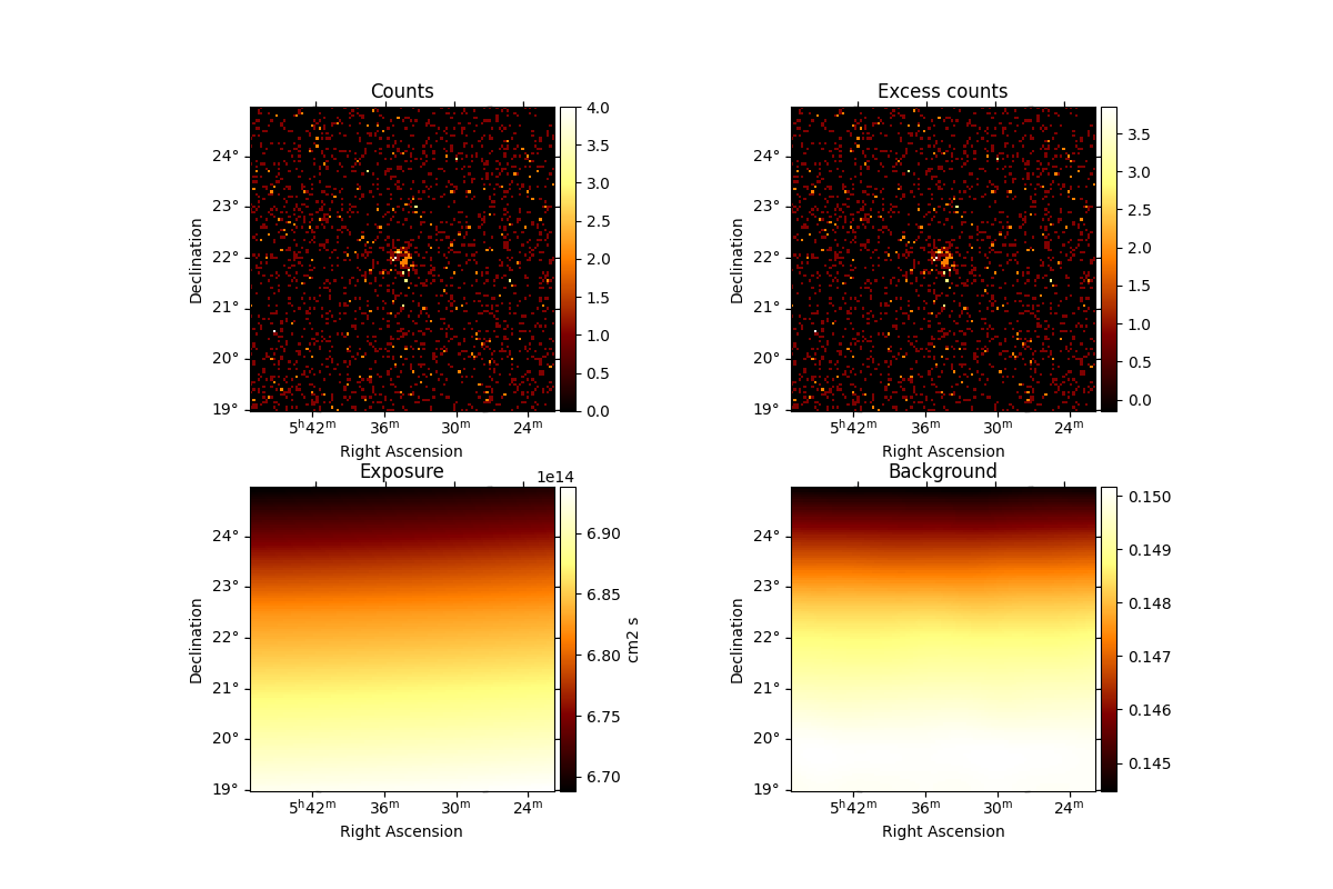
Check the dataset we produced

We will now check the contents of the dataset. We can use the .peek() method to quickly get a glimpse of the contents

dataset.peek()
plt.show()

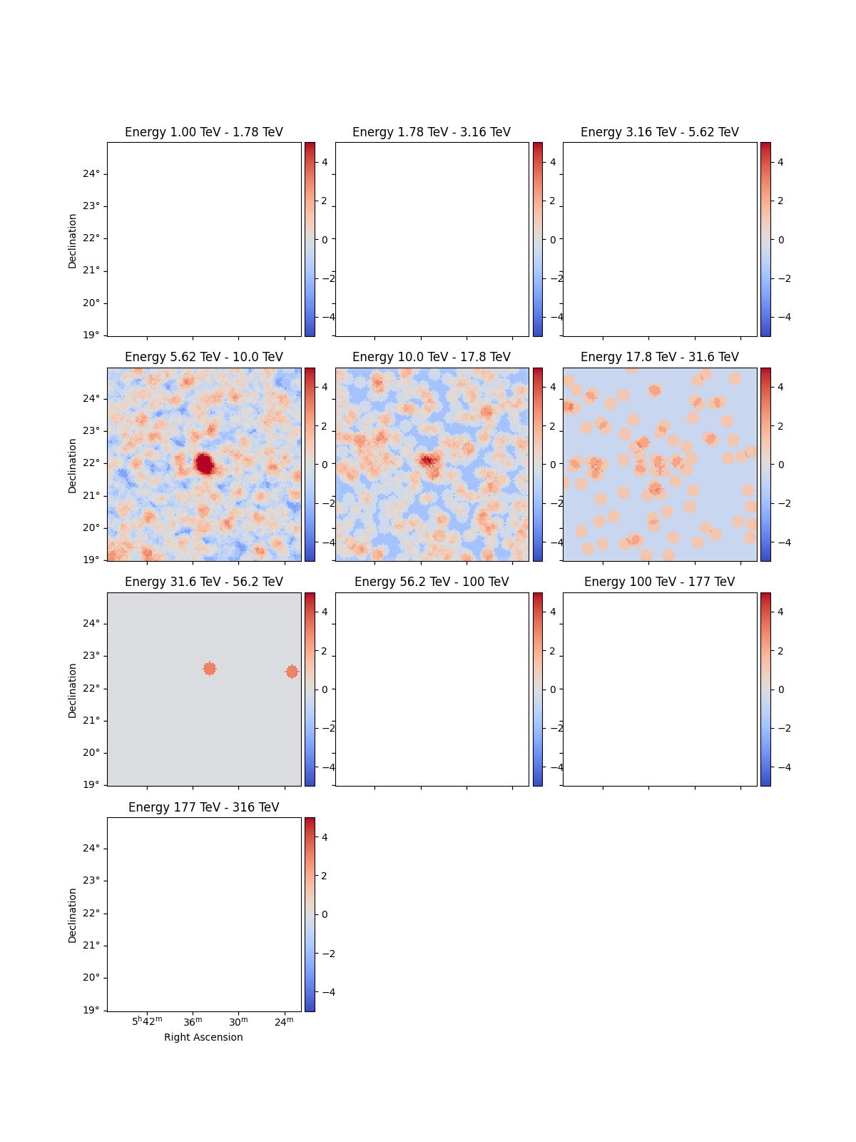
Create significance maps to check that the Crab is visible:

excess_estimator = ExcessMapEstimator(
    correlation_radius="0.2 deg", selection_optional=[], energy_edges=energy_axis.edges
)
excess = excess_estimator.run(dataset)

(dataset.mask * excess["sqrt_ts"]).plot_grid(
    add_cbar=True, cmap="coolwarm", vmin=-5, vmax=5
)
plt.show()

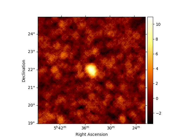
Combining all energies

excess_estimator_integrated = ExcessMapEstimator(
    correlation_radius="0.2 deg", selection_optional=[]
)
excess_integrated = excess_estimator_integrated.run(dataset)

excess_integrated["sqrt_ts"].plot(add_cbar=True)
plt.show()

Exercises

• Repeat the process for a different fHit bin.

• Repeat the process for all the fHit bins provided in the data release and fit a model to the result.

Next steps

Now you know how to access and work with HAWC data. All other tutorials and documentation concerning 3D analysis techniques and the MapDataset object can be used from this step on.