Note
Go to the end to download the full example code or to run this example in your browser via Binder.
Source detection and significance maps#
Build a list of significant excesses in a Fermi-LAT map.
Context#
The first task in a source catalog production is to identify significant excesses in the data that can be associated to unknown sources and provide a preliminary parametrization in terms of position, extent, and flux. In this notebook we will use Fermi-LAT data to illustrate how to detect candidate sources in counts images with known background.
Objective: build a list of significant excesses in a Fermi-LAT map
Proposed approach#
This notebook show how to do source detection with Gammapy using the
methods available in estimators. We will use images from a
Fermi-LAT 3FHL high-energy Galactic center dataset to do this:
perform adaptive smoothing on counts image
produce 2-dimensional test-statistics (TS)
run a peak finder to detect point-source candidates
compute Li & Ma significance images
estimate source candidates radius and excess counts
Note that what we do here is a quick-look analysis, the production of real source catalogs use more elaborate procedures.
We will work with the following functions and classes:
Setup#
As always, let’s get started with some setup …
import numpy as np
import astropy.units as u

# %matplotlib inline
import matplotlib.pyplot as plt
from IPython.display import display
from gammapy.datasets import MapDataset
from gammapy.estimators import ASmoothMapEstimator, TSMapEstimator
from gammapy.estimators.utils import find_peaks, find_peaks_in_flux_map
from gammapy.irf import EDispKernelMap, PSFMap
from gammapy.maps import Map
from gammapy.modeling.models import PointSpatialModel, PowerLawSpectralModel, SkyModel
Read in input images#
We first read the relevant maps:
counts = Map.read("$GAMMAPY_DATA/fermi-3fhl-gc/fermi-3fhl-gc-counts-cube.fits.gz")
background = Map.read(
    "$GAMMAPY_DATA/fermi-3fhl-gc/fermi-3fhl-gc-background-cube.fits.gz"
)

exposure = Map.read("$GAMMAPY_DATA/fermi-3fhl-gc/fermi-3fhl-gc-exposure-cube.fits.gz")

psfmap = PSFMap.read(
    "$GAMMAPY_DATA/fermi-3fhl-gc/fermi-3fhl-gc-psf-cube.fits.gz",
    format="gtpsf",
)

edisp = EDispKernelMap.from_diagonal_response(
    energy_axis=counts.geom.axes["energy"],
    energy_axis_true=exposure.geom.axes["energy_true"],
)

dataset = MapDataset(
    counts=counts,
    background=background,
    exposure=exposure,
    psf=psfmap,
    name="fermi-3fhl-gc",
    edisp=edisp,
)
/home/runner/work/gammapy-docs/gammapy-docs/gammapy/.tox/build_docs/lib/python3.12/site-packages/astropy/wcs/wcs.py:919: FITSFixedWarning: 'datfix' made the change 'Set DATEREF to '2001-01-01T00:01:04.184' from MJDREF.
Set MJD-OBS to 54682.655283 from DATE-OBS.
Set MJD-END to 57236.967546 from DATE-END'.
  warnings.warn(
Adaptive smoothing#
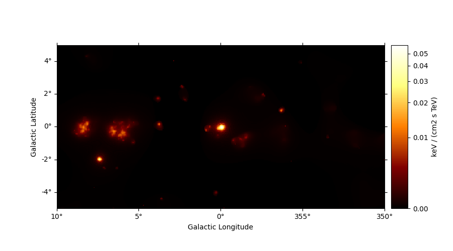
For visualisation purpose it can be nice to look at a smoothed counts image. This can be performed using the adaptive smoothing algorithm from Ebeling et al. (2006).
In the following example the threshold
argument gives the minimum significance expected, values below are clipped.
scales = u.Quantity(np.arange(0.05, 1, 0.05), unit="deg")
smooth = ASmoothMapEstimator(threshold=3, scales=scales, energy_edges=[10, 500] * u.GeV)
images = smooth.run(dataset)

plt.figure(figsize=(9, 5))
images["flux"].plot(add_cbar=True, stretch="asinh")
plt.show()
TS map estimation#
The Test Statistic, \(TS = 2 \Delta log L\) (Mattox et al. 1996), compares the likelihood function L optimized with and without a given source. The TS map is computed by fitting a single amplitude parameter on each pixel as described in Appendix A of Stewart (2009). The fit is simplified by finding roots of the derivative of the fit statistics (default settings use Brent’s method).
We first need to define the model that will be used to test for the existence of a source. Here, we use a point source.
spatial_model = PointSpatialModel()

# We choose units consistent with the map units here...
spectral_model = PowerLawSpectralModel(amplitude="1e-22 cm-2 s-1 keV-1", index=2)
kernel_model = SkyModel(spatial_model=spatial_model, spectral_model=spectral_model)
Here we show a full configuration of the estimator. We remind the user of the meaning of the various quantities:
model: aSkyModelwhich is converted to a source model kernelkernel_width: the width for the above kerneln_sigma: number of sigma for the flux errorn_sigma_ul: the number of sigma for the flux upper limitsselection_optional: what optional maps to computen_jobs: for running in parallel, the number of processes used for the computationsum_over_energy_groups: to sum over the energy groups or fit thenormon the full energy cube
estimator = TSMapEstimator(
    kernel_model=kernel_model,
    kernel_width="1 deg",
    energy_edges=[10, 500] * u.GeV,
    n_sigma=1,
    n_sigma_ul=2,
    selection_optional=None,
    n_jobs=1,
    sum_over_energy_groups=True,
)


maps = estimator.run(dataset)
Accessing and visualising results#
Below we print the result of the TSMapEstimator. We have access to a number of
different quantities, as shown below. We can also access the quantities names
through maps.available_quantities.
print(maps)
FluxMaps
--------

  geom                   : WcsGeom
  axes                   : ['lon', 'lat', 'energy']
  shape                  : (np.int64(400), np.int64(200), 1)
  quantities             : ['ts', 'norm', 'niter', 'norm_err', 'npred', 'npred_excess', 'stat', 'stat_null', 'success']
  ref. model             : pl
  n_sigma                : 1
  n_sigma_ul             : 2
  sqrt_ts_threshold_ul   : 2
  sed type init          : likelihood
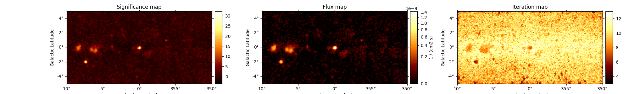
fig, (ax1, ax2, ax3) = plt.subplots(
    ncols=3,
    figsize=(20, 3),
    subplot_kw={"projection": counts.geom.wcs},
    gridspec_kw={"left": 0.1, "right": 0.98},
)

maps["sqrt_ts"].plot(ax=ax1, add_cbar=True)
ax1.set_title("Significance map")
maps["flux"].plot(ax=ax2, add_cbar=True, stretch="sqrt", vmin=0)
ax2.set_title("Flux map")
maps["niter"].plot(ax=ax3, add_cbar=True)
ax3.set_title("Iteration map")
plt.show()
The flux in each pixel is obtained by multiplying a reference model with a normalisation factor:
print(maps.reference_model)
SkyModel

  Name                      : 6Vs8EIq_
  Datasets names            : None
  Spectral model type       : PowerLawSpectralModel
  Spatial  model type       : PointSpatialModel
  Temporal model type       :
  Parameters:
    index                         :      2.000   +/-    0.00
    amplitude                     :   1.00e-22   +/- 0.0e+00 1 / (keV s cm2)
    reference             (frozen):      1.000       TeV
    lon_0                         :      0.000   +/-    0.00 deg
    lat_0                         :      0.000   +/-    0.00 deg
maps.norm.plot(add_cbar=True, stretch="sqrt")
plt.show()

Source candidates#
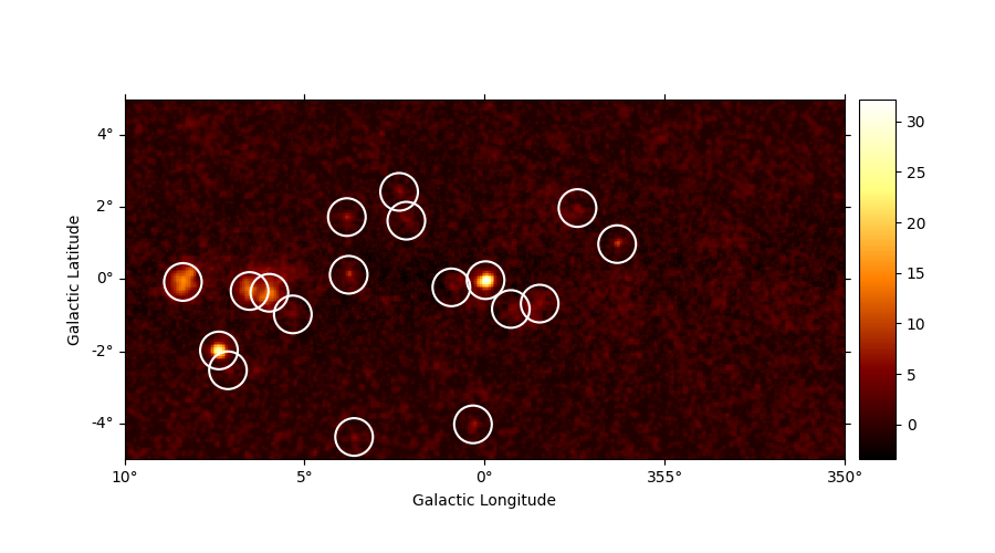
Let’s run a peak finder on the sqrt_ts image to get a list of
point-sources candidates (positions and peak sqrt_ts values). The
find_peaks function performs a local maximum search in a sliding
window, the argument min_distance is the minimum pixel distance
between peaks (smallest possible value and default is 1 pixel).
sources = find_peaks(maps["sqrt_ts"], threshold=5, min_distance="0.25 deg")
nsou = len(sources)
display(sources)

# Plot sources on top of significance sky image
plt.figure(figsize=(9, 5))
ax = maps["sqrt_ts"].plot(add_cbar=True)

ax.scatter(
    sources["ra"],
    sources["dec"],
    transform=ax.get_transform("icrs"),
    color="none",
    edgecolor="w",
    marker="o",
    s=600,
    lw=1.5,
)
plt.show()
value   x   y      ra       dec
                  deg       deg
------ --- --- --------- ---------
31.361 200  99 266.41449 -28.97054
27.565  52  60 272.43197 -23.54282
14.302  32  99 271.11366 -21.72027
13.422  69  93 270.40919 -23.47797
    13  80  92 270.15899 -23.98049
9.7135 273 119 263.18257 -31.52587
8.6615 124 102 268.46711 -25.63326
7.2674 123 134 266.97596 -24.77174
6.7151 193  19 270.59696 -30.69138
6.1638 152 148 265.48068 -25.64323
5.7289 127  12 272.77351 -27.97934
5.6195 251 139 262.90685 -30.05853
5.5232 230  85 266.20093 -30.61539
5.3338 181  95 267.17020 -28.26173
5.2454 214  83 266.78188 -29.98429
5.1981 223  85 266.41273 -30.31680
5.0083  57  49 272.82739 -24.02653
5.0049 156 132 266.12148 -26.23306
We can also utilise find_peaks_in_flux_map
to display various parameters from the FluxMaps
sources_flux_map = find_peaks_in_flux_map(maps, threshold=5, min_distance="0.25 deg")
display(sources_flux_map)
 x   y      ra       dec    ... stat_null  success     flux      flux_err
           deg       deg    ...                    1 / (s cm2) 1 / (s cm2)
--- --- --------- --------- ... ---------- ------- ----------- -----------
156 132 266.12148 -26.23306 ...  692.59451    True   5.436e-11   1.788e-11
 57  49 272.82739 -24.02653 ...  723.70546    True   5.192e-11   1.678e-11
223  85 266.41273 -30.31680 ...  878.61418    True   9.687e-11   2.735e-11
214  83 266.78188 -29.98429 ...  838.88781    True   8.749e-11   2.451e-11
181  95 267.17020 -28.26173 ...  659.39224    True   1.167e-10   3.003e-11
230  85 266.20093 -30.61539 ...  871.72523    True   1.003e-10   2.723e-11
251 139 262.90685 -30.05853 ...  766.22149    True   6.209e-11   1.846e-11
127  12 272.77351 -27.97934 ...  433.37517    True   3.982e-11   1.323e-11
152 148 265.48068 -25.64323 ...  611.76473    True   6.707e-11   1.828e-11
193  19 270.59696 -30.69138 ...  445.28958    True   6.361e-11   1.684e-11
123 134 266.97596 -24.77174 ...  655.77218    True   8.763e-11   2.078e-11
124 102 268.46711 -25.63326 ...  881.98258    True   1.603e-10   2.958e-11
273 119 263.18257 -31.52587 ...  846.92490    True   1.687e-10   2.885e-11
 80  92 270.15899 -23.98049 ... 1093.46225    True   4.124e-10   5.080e-11
 69  93 270.40919 -23.47797 ... 1044.25763    True   4.113e-10   5.055e-11
 32  99 271.11366 -21.72027 ... 1035.91218    True   4.783e-10   5.534e-11
 52  60 272.43197 -23.54282 ... 1092.41995    True   5.890e-10   4.652e-11
200  99 266.41449 -28.97054 ...  137.30287    True   1.354e-09   7.791e-11
Note that we used the instrument point-spread-function (PSF) as kernel, so the hypothesis we test is the presence of a point source. In order to test for extended sources we would have to use as kernel an extended template convolved by the PSF. Alternatively, we can compute the significance of an extended excess using the Li & Ma formalism, which is faster as no fitting is involved.
What next?#
In this notebook, we have seen how to work with images and compute TS and significance images from counts data, if a background estimate is already available.
Here’s some suggestions what to do next:
Look how background estimation is performed for IACTs with and without the high level interface in High level interface and Low level API notebooks, respectively
Learn about 2D model fitting in the 2D map fitting notebook
Find more about Fermi-LAT data analysis in the Fermi-LAT with Gammapy notebook
Use source candidates to build a model and perform a 3D fitting (see 3D detailed analysis, Multi instrument joint 3D and 1D analysis notebooks for some hints)
Total running time of the script: (0 minutes 12.398 seconds)