Note
Go to the end to download the full example code or to run this example in your browser via Binder.
Sample a source with energy-dependent temporal evolution#
This notebook shows how to sample events of sources whose model evolves in energy and time.
Prerequisites#
To understand how to generate a model and a MapDataset and how to fit the data, please refer to
the SkyModel and 3D map simulation tutorial.
To know how to sample events for standards sources, we suggest to visit the event sampler
Event sampling tutorial.
Objective#
Describe the process of sampling events of a source having an energy-dependent temporal model, and obtain an output event-list.
Proposed approach#
Here we will show how to create an energy dependent temporal model; then we also create an observation and define a Dataset object. Finally, we describe how to sample events from the given model.
We will work with the following functions and classes:
Setup#
As usual, let’s start with some general imports…
from pathlib import Path
import astropy.units as u
from astropy.coordinates import Angle, SkyCoord
from astropy.time import Time
from regions import CircleSkyRegion, PointSkyRegion
import matplotlib.pyplot as plt
from gammapy.data import FixedPointingInfo, Observation, observatory_locations
from gammapy.datasets import MapDataset, MapDatasetEventSampler
from gammapy.irf import load_irf_dict_from_file
from gammapy.makers import MapDatasetMaker
from gammapy.maps import MapAxis, RegionNDMap, WcsGeom
from gammapy.modeling.models import (
    ConstantSpectralModel,
    FoVBackgroundModel,
    LightCurveTemplateTemporalModel,
    PointSpatialModel,
    PowerLawSpectralModel,
    SkyModel,
)
Create the energy-dependent temporal model#
The source we want to simulate has a spectrum that varies as a function of the time. Here we show how to create an energy dependent temporal model. If you already have such a model, go directly to the corresponding section.
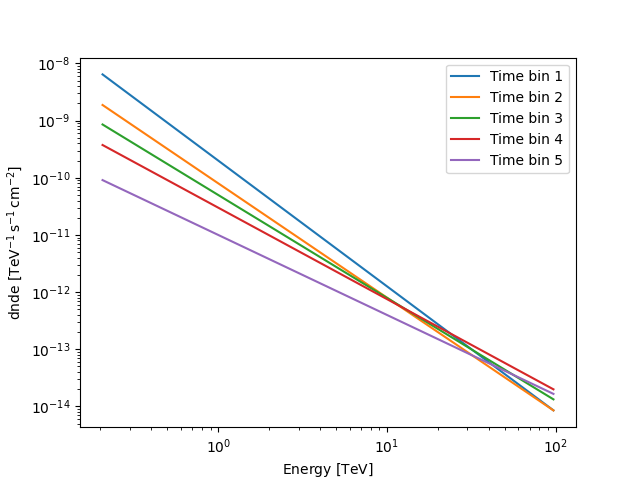
In the following example, the source spectrum will vary continuously with time. Here we define 5 time bins and represent the spectrum at the center of each bin as a powerlaw. The spectral evolution is also shown in the following plot:
amplitudes = u.Quantity(
    [2e-10, 8e-11, 5e-11, 3e-11, 1e-11], unit="cm-2s-1TeV-1"
)  # amplitude
indices = u.Quantity([2.2, 2.0, 1.8, 1.6, 1.4], unit="")  # index

for i in range(len(amplitudes)):
    spec = PowerLawSpectralModel(
        index=indices[i], amplitude=amplitudes[i], reference="1 TeV"
    )
    spec.plot([0.2, 100] * u.TeV, label=f"Time bin {i + 1}")
plt.legend()
plt.show()
/home/runner/work/gammapy-docs/gammapy-docs/gammapy/.tox/build_docs/lib/python3.12/site-packages/gammapy/modeling/models/spectral.py:649: UserWarning: This axis already has a converter set and is updating to a potentially incompatible converter
  ax.plot(energy.center, flux.quantity[:, 0, 0], **kwargs)
Let’s now create the temporal model (if you already have this model,
please go directly to the Read the energy-dependent model section),
that will be defined as a LightCurveTemplateTemporalModel. The latter
take as input a RegionNDMap with temporal and energy axes, on which
the fluxes are stored.
To create such map, we first need to define a time axis with MapAxis:
here we consider 5 time bins of 720 s (i.e. 1 hr in total).
As a second step, we create an energy axis with 10 bins where the
powerlaw spectral models will be evaluated.
pointing_position = SkyCoord("100 deg", "30 deg", frame="icrs")
position = FixedPointingInfo(fixed_icrs=pointing_position.icrs)

time_axis = MapAxis.from_bounds(0 * u.s, 3600 * u.s, nbin=5, name="time", interp="lin")

energy_axis = MapAxis.from_energy_bounds(
    energy_min=0.2 * u.TeV, energy_max=100 * u.TeV, nbin=10
)
Now let’s create the RegionNDMap and fill it with the expected
spectral values:
m = RegionNDMap.create(
    region=PointSkyRegion(center=pointing_position),
    axes=[energy_axis, time_axis],
    unit="cm-2s-1TeV-1",
)
to compute the spectra as a function of time we extract the coordinates of the geometry
coords = m.geom.get_coord(sparse=True)
We reshape the indices and amplitudes array to perform broadcasting
indices = indices.reshape(coords["time"].shape)
amplitudes = amplitudes.reshape(coords["time"].shape)
evaluate the spectra and fill the RegionNDMap
m.quantity = PowerLawSpectralModel.evaluate(
    coords["energy"], indices, amplitudes, 1 * u.TeV
)
Create the temporal model and write it to disk#
Now, we define the LightCurveTemplateTemporalModel. It needs the
map we created above and a reference time. The latter
is crucial to evaluate the model as a function of time.
We show also how to write the model on disk, noting that we explicitly
set the format to map.
Read the energy-dependent model#
We read the map written on disc again with read().
When the model is from a map, the arguments format="map" is mandatory.
The map is fits file, with 3 extensions:
1)
SKYMAP: a table with aCHANNELandDATAcolumn; the number of rows is given by the product of the energy and time bins. TheDATArepresent the values of the model at each energy;2)
SKYMAP_BANDS: a table withCHANNEL,ENERGY,E_MIN,E_MAX,TIME,TIME_MINandTIME_MAX.ENERGYis the mean ofE_MINandE_MAX, as well asTIMEis the mean ofTIME_MINandTIME_MAX; this extension should contain the reference time in the header, through the keywordsMJDREFIandMJDREFF.3)
SKYMAP_REGION: it gives information on the spatial morphology, i.e.SHAPE(onlypointis accepted),XandY(source position),R(the radius if extended; not used in our case) andROTANG(the angular rotation of the spatial model, if extended; not used in our case).
temporal_model = LightCurveTemplateTemporalModel.read(filename, format="map")
We note that an interpolation scheme is also provided when loading
a map: for an energy-dependent temporal model, the method and
values_scale arguments by default are set to linear and log.
We warn the reader to carefully check the interpolation method used
for the time axis while creating the template model, as different
methods provide different results.
By default, we assume linear interpolation for the time, log
for the energies and values.
Users can modify the method and values_scale arguments but we
warn that this should be done only when the user knows the consequences
of the changes. Here, we show how to set them explicitly:
temporal_model.method = "linear"  # default
temporal_model.values_scale = "log"  # default
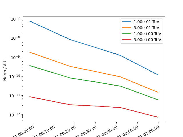
We can have a visual inspection of the temporal model at different energies:
time_range = temporal_model.reference_time + [-100, 3600] * u.s

temporal_model.plot(time_range=time_range, energy=[0.1, 0.5, 1, 5] * u.TeV)
plt.semilogy()
plt.show()
Prepare and run the event sampler#
Define the simulation source model#
Now that the temporal model is complete, we create the whole source
SkyModel. We define its spatial morphology as point-like. This
is a mandatory condition to simulate energy-dependent temporal model.
Other morphologies will raise an error!
Note also that the source spectral_model is a ConstantSpectralModel:
this is necessary and mandatory, as the real source spectrum is actually
passed through the map.
spatial_model = PointSpatialModel.from_position(pointing_position)
spectral_model = ConstantSpectralModel(const="1 cm-2 s-1 TeV-1")

model = SkyModel(
    spatial_model=spatial_model,
    spectral_model=spectral_model,
    temporal_model=temporal_model,
    name="test-source",
)

bkg_model = FoVBackgroundModel(dataset_name="my-dataset")

models = [model, bkg_model]
Define an observation and make a dataset#
In the following, we define an observation of 1 hr with CTAO in the
alpha-configuration for the south array, and we also create a dataset
to be passed to the event sampler. The full SkyModel
created above is passed to the dataset.
path = Path("$GAMMAPY_DATA/cta-caldb")
irf_filename = "Prod5-South-20deg-AverageAz-14MSTs37SSTs.180000s-v0.1.fits.gz"

pointing_position = SkyCoord(ra=100 * u.deg, dec=30 * u.deg)
pointing = FixedPointingInfo(fixed_icrs=pointing_position)
livetime = 1 * u.hr

irfs = load_irf_dict_from_file(path / irf_filename)
location = observatory_locations["ctao_south"]

observation = Observation.create(
    obs_id=1001,
    pointing=pointing,
    livetime=livetime,
    irfs=irfs,
    location=location,
)
energy_axis = MapAxis.from_energy_bounds("0.2 TeV", "100 TeV", nbin=5, per_decade=True)
energy_axis_true = MapAxis.from_energy_bounds(
    "0.05 TeV", "150 TeV", nbin=10, per_decade=True, name="energy_true"
)
migra_axis = MapAxis.from_bounds(0.5, 2, nbin=150, node_type="edges", name="migra")

geom = WcsGeom.create(
    skydir=pointing_position,
    width=(2, 2),
    binsz=0.02,
    frame="icrs",
    axes=[energy_axis],
)
empty = MapDataset.create(
    geom,
    energy_axis_true=energy_axis_true,
    migra_axis=migra_axis,
    name="my-dataset",
)
maker = MapDatasetMaker(selection=["exposure", "background", "psf", "edisp"])
dataset = maker.run(empty, observation)

dataset.models = models

print(dataset.models)
DatasetModels

Component 0: SkyModel

  Name                      : test-source
  Datasets names            : None
  Spectral model type       : ConstantSpectralModel
  Spatial  model type       : PointSpatialModel
  Temporal model type       : LightCurveTemplateTemporalModel
  Parameters:
    const                         :      1.000   +/-    0.00 1 / (TeV s cm2)
    lon_0                         :    100.000   +/-    0.00 deg
    lat_0                         :     30.000   +/-    0.00 deg
    t_ref                 (frozen):  51544.000       d

Component 1: FoVBackgroundModel

  Name                      : my-dataset-bkg
  Datasets names            : ['my-dataset']
  Spectral model type       : PowerLawNormSpectralModel
  Parameters:
    tilt                  (frozen):      0.000
    norm                          :      1.000   +/-    0.00
    reference             (frozen):      1.000       TeV
Let’s simulate the model#
Initialize and run the MapDatasetEventSampler class. We also define
the oversample_energy_factor arguments: this should be carefully
considered by the user, as a higher oversample_energy_factor gives
a more precise source flux estimate, at the expense of computational
time. Here we adopt an oversample_energy_factor of 10:
sampler = MapDatasetEventSampler(random_state=0, oversample_energy_factor=10)
events = sampler.run(dataset, observation)
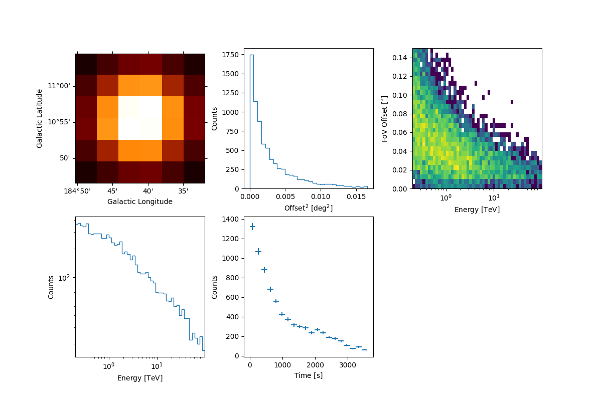
Let’s inspect the simulated events in the source region:
src_position = SkyCoord(100.0, 30.0, frame="icrs", unit="deg")

on_region_radius = Angle("0.15 deg")
on_region = CircleSkyRegion(center=src_position, radius=on_region_radius)

src_events = events.select_region(on_region)

src_events.peek()
plt.show()
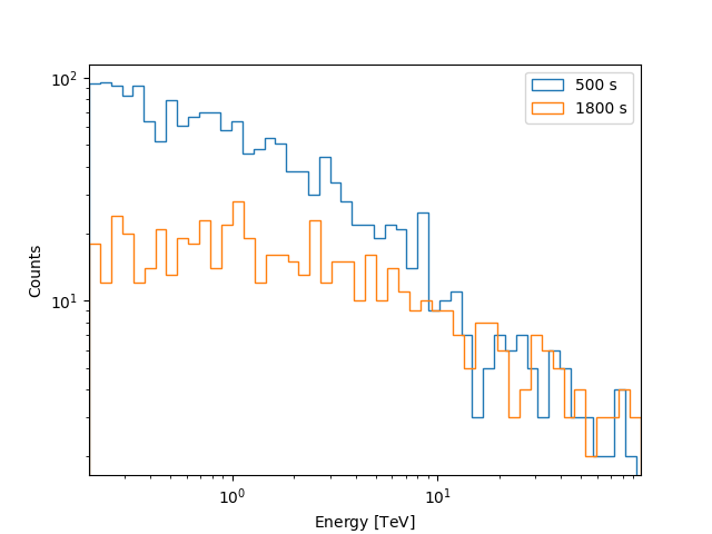
Let’s inspect the simulated events as a function of time:
time_interval = temporal_model.reference_time + [300, 700] * u.s
src_events.select_time(time_interval).plot_energy(label="500 s")

time_interval = temporal_model.reference_time + [1600, 2000] * u.s
src_events.select_time(time_interval).plot_energy(label="1800 s")

plt.legend()
plt.show()
Exercises#
Try to create a temporal model with a more complex energy-dependent evolution;
Read your temporal model in Gammapy and simulate it;