Note
Go to the end to download the full example code or to run this example in your browser via Binder.
Low level API#
Introduction to Gammapy analysis using the low level API.
Prerequisites#
Understanding the gammapy data workflow, in particular what are DL3 events and instrument response functions (IRF).
Understanding of the data reduction and modeling fitting process as shown in the analysis with the high level interface tutorial High level interface
Context#
This notebook is an introduction to gammapy analysis this time using the lower level classes and functions the library. This allows to understand what happens during two main gammapy analysis steps, data reduction and modeling/fitting.
Objective: Create a 3D dataset of the Crab using the H.E.S.S. DL3 data release 1 and perform a simple model fitting of the Crab nebula using the lower level gammapy API.
Proposed approach#
Here, we have to interact with the data archive (with the
DataStore) to retrieve a list of selected observations
(Observations). Then, we define the geometry of the
MapDataset object we want to produce and the maker
object that reduce an observation to a dataset.
We can then proceed with data reduction with a loop over all selected observations to produce datasets in the relevant geometry and stack them together (i.e.sum them all).
In practice, we have to:
Create a
DataStorepointing to the relevant dataApply an observation selection to produce a list of observations, a
Observationsobject.Define a geometry of the Map we want to produce, with a sky projection and an energy range.
Create a
MapAxisfor the energyCreate a
WcsGeomfor the geometryCreate the necessary makers:
the map dataset maker
MapDatasetMakerthe background normalization maker, here a
FoVBackgroundMakerand usually the safe range maker :
SafeMaskMaker
Perform the data reduction loop. And for every observation:
Apply the makers sequentially to produce the current
MapDatasetStack it on the target one.
Define the
SkyModelto apply to the dataset.Create a
Fitobject and run it to fit the model parametersApply a
FluxPointsEstimatorto compute flux points for the spectral part of the fit.
Setup#
First, we setup the analysis by performing required imports.
from pathlib import Path
from astropy import units as u
from astropy.coordinates import SkyCoord
from regions import CircleSkyRegion

# %matplotlib inline
import matplotlib.pyplot as plt
from gammapy.data import DataStore
from gammapy.datasets import MapDataset
from gammapy.estimators import FluxPointsEstimator
from gammapy.makers import FoVBackgroundMaker, MapDatasetMaker, SafeMaskMaker
from gammapy.maps import MapAxis, WcsGeom
from gammapy.modeling import Fit
from gammapy.modeling.models import (
    FoVBackgroundModel,
    PointSpatialModel,
    PowerLawSpectralModel,
    SkyModel,
)
from gammapy.utils.check import check_tutorials_setup
from gammapy.visualization import plot_npred_signal
Check setup#
check_tutorials_setup()
System:

        python_executable      : /home/runner/work/gammapy-docs/gammapy-docs/gammapy/.tox/build_docs/bin/python
        python_version         : 3.12.13
        machine                : x86_64
        system                 : Linux


Gammapy package:

        version                : 2.0.dev4000+g6ed4106cb
        path                   : /home/runner/work/gammapy-docs/gammapy-docs/gammapy/.tox/build_docs/lib/python3.12/site-packages/gammapy


Other packages:

        numpy                  : 2.4.6
        scipy                  : 1.17.1
        astropy                : 7.2.2
        regions                : 0.11
        click                  : 8.4.2
        PyYAML                 : 6.0.3
        pydantic               : 2.13.4
        IPython                : 9.15.0
        jupyter                : not installed
        jupyterlab             : not installed
        matplotlib             : 3.11.1
        pandas                 : 3.0.3
        healpy                 : 1.19.0
        iminuit                : 2.32.0
        sherpa                 : 4.18.0
        naima                  : 0.10.3
        emcee                  : 3.1.6
        corner                 : 2.3.0
        ray                    : 2.54.1


Gammapy environment variables:

        GAMMAPY_DATA           : /home/runner/work/gammapy-docs/gammapy-docs/gammapy-datasets/dev
Defining the datastore and selecting observations#
We first use the DataStore object to access the
observations we want to analyse. Here the H.E.S.S. DL3 DR1.
data_store = DataStore.from_dir("$GAMMAPY_DATA/hess-dl3-dr1")
We can now define an observation filter to select only the relevant observations. Here we use a cone search which we define with a python dict.
We then filter the ObservationTable with
select_observations.
selection = dict(
    type="sky_circle",
    frame="icrs",
    lon="83.633 deg",
    lat="22.014 deg",
    radius="5 deg",
)
selected_obs_table = data_store.obs_table.select_observations(selection)
We can now retrieve the relevant observations by passing their
obs_id to the get_observations
method.
observations = data_store.get_observations(selected_obs_table["OBS_ID"])
Preparing reduced datasets geometry#
Now we define a reference geometry for our analysis, We choose a WCS based geometry with a binsize of 0.02 deg and also define an energy axis:
energy_axis = MapAxis.from_energy_bounds(1.0, 10.0, 4, unit="TeV")

geom = WcsGeom.create(
    skydir=(83.633, 22.014),
    binsz=0.02,
    width=(2, 2),
    frame="icrs",
    proj="CAR",
    axes=[energy_axis],
)

# Reduced IRFs are defined in true energy (i.e. not measured energy).
energy_axis_true = MapAxis.from_energy_bounds(
    0.5, 20, 10, unit="TeV", name="energy_true"
)
Now we can define the target dataset with this geometry.
stacked = MapDataset.create(
    geom=geom, energy_axis_true=energy_axis_true, name="crab-stacked"
)
Data reduction#
Create the maker classes to be used#
The MapDatasetMaker object is initialized as well as
the SafeMaskMaker that carries here a maximum offset
selection. The FoVBackgroundMaker utilised here has the
default spectral_model but it is possible to set your own. For further
details see the FoV background.
offset_max = 2.5 * u.deg
maker = MapDatasetMaker()
maker_safe_mask = SafeMaskMaker(
    methods=["offset-max", "aeff-max"], offset_max=offset_max
)

circle = CircleSkyRegion(center=SkyCoord("83.63 deg", "22.14 deg"), radius=0.2 * u.deg)
exclusion_mask = ~geom.region_mask(regions=[circle])
maker_fov = FoVBackgroundMaker(method="fit", exclusion_mask=exclusion_mask)
Perform the data reduction loop#
for obs in observations:
    # First a cutout of the target map is produced
    cutout = stacked.cutout(
        obs.get_pointing_icrs(obs.tmid), width=2 * offset_max, name=f"obs-{obs.obs_id}"
    )
    # A MapDataset is filled in this cutout geometry
    dataset = maker.run(cutout, obs)
    # The data quality cut is applied
    dataset = maker_safe_mask.run(dataset, obs)
    # fit background model
    dataset = maker_fov.run(dataset)
    print(
        f"Background norm obs {obs.obs_id}: {dataset.background_model.spectral_model.norm.value:.2f}"
    )
    # The resulting dataset cutout is stacked onto the final one
    stacked.stack(dataset)

print(stacked)
Background norm obs 23523: 0.99
Background norm obs 23526: 1.08
Background norm obs 23559: 0.99
Background norm obs 23592: 1.10
MapDataset
----------

  Name                            : crab-stacked

  Total counts                    : 2479
  Total background counts         : 2112.97
  Total excess counts             : 366.03

  Predicted counts                : 2112.97
  Predicted background counts     : 2112.97
  Predicted excess counts         : nan

  Exposure min                    : 3.75e+08 m2 s
  Exposure max                    : 3.48e+09 m2 s

  Number of total bins            : 40000
  Number of fit bins              : 40000

  Fit statistic type              : cash
  Fit statistic value (-2 log(L)) : nan

  Number of models                : 0
  Number of parameters            : 0
  Number of free parameters       : 0
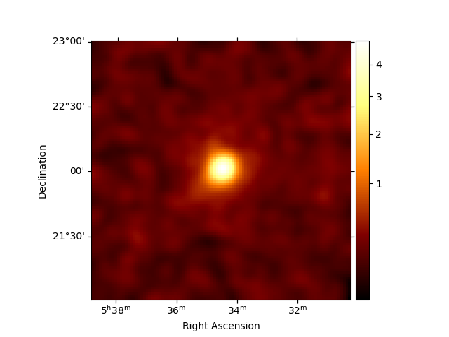
Inspect the reduced dataset#
stacked.counts.sum_over_axes().smooth(0.05 * u.deg).plot(stretch="sqrt", add_cbar=True)
plt.show()
Save dataset to disk#
It is common to run the preparation step independent of the likelihood fit, because often the preparation of maps, PSF and energy dispersion is slow if you have a lot of data. We first create a folder:
path = Path("analysis_2")
path.mkdir(exist_ok=True)
And then write the maps and IRFs to disk by calling the dedicated
write method:
filename = path / "crab-stacked-dataset.fits.gz"
stacked.write(filename, overwrite=True)
Define the model#
We first define the model, a SkyModel, as the combination of a point
source SpatialModel with a powerlaw SpectralModel:
target_position = SkyCoord(ra=83.63308, dec=22.01450, unit="deg")
spatial_model = PointSpatialModel(
    lon_0=target_position.ra, lat_0=target_position.dec, frame="icrs"
)

spectral_model = PowerLawSpectralModel(
    index=2.702,
    amplitude=4.712e-11 * u.Unit("1 / (cm2 s TeV)"),
    reference=1 * u.TeV,
)

sky_model = SkyModel(
    spatial_model=spatial_model, spectral_model=spectral_model, name="crab"
)

bkg_model = FoVBackgroundModel(dataset_name="crab-stacked")
Now we assign this model to our reduced dataset:
Fit the model#
The Fit class is orchestrating the fit, connecting
the stats method of the dataset to the minimizer. By default, it
uses iminuit.
It is possible that the fit will try to converge on an unrelated position therefore you may choose to constrain the model parameter ranges to stay within your expected region (see here). For further information on fitting you can see the Fitting overview tutorial or this section about modifying your parameters.
The fit constructor takes dictionaries that define global options for the optimizer.
The FitResult contains information about the optimization and
parameter error calculation.
print(result)
OptimizeResult

        backend    : minuit
        method     : migrad
        success    : True
        message    : Optimization terminated successfully.
        nfev       : 124
        total stat : 16240.82

CovarianceResult

        backend    : minuit
        method     : hesse
        success    : True
        message    : Hesse terminated successfully.
The fitted parameters are visible from the
Models object.
print(stacked.models.to_parameters_table())
     model       type    name     value    ...    max    frozen link prior
---------------- ---- --------- ---------- ... --------- ------ ---- -----
            crab          index 2.6024e+00 ...       nan  False
            crab      amplitude 4.5921e-11 ...       nan  False
            crab      reference 1.0000e+00 ...       nan   True
            crab          lon_0 8.3619e+01 ...       nan  False
            crab          lat_0 2.2024e+01 ... 9.000e+01  False
crab-stacked-bkg           tilt 0.0000e+00 ...       nan   True
crab-stacked-bkg           norm 9.3513e-01 ...       nan  False
crab-stacked-bkg      reference 1.0000e+00 ...       nan   True
Here we can plot the number of predicted counts for each model and
for the background in our dataset. In order to do this, we can use
the plot_npred_signal function.
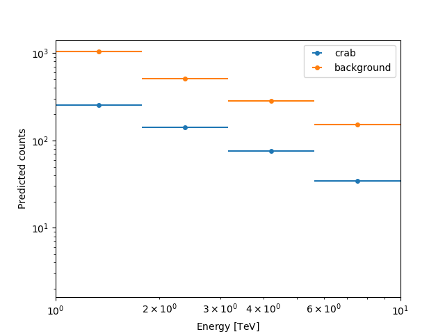
/home/runner/work/gammapy-docs/gammapy-docs/gammapy/.tox/build_docs/lib/python3.12/site-packages/gammapy/maps/region/ndmap.py:154: UserWarning: This axis already has a converter set and is updating to a potentially incompatible converter
  ax.errorbar(
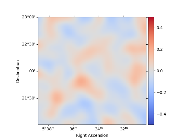
Inspecting residuals#
For any fit it is useful to inspect the residual images. We have a few
options on the dataset object to handle this. First we can use
plot_residuals_spatial to plot a residual image, summed over all
energies:
stacked.plot_residuals_spatial(method="diff/sqrt(model)", vmin=-0.5, vmax=0.5)
plt.show()
In addition, we can also specify a region in the map to show the spectral residuals:
region = CircleSkyRegion(center=SkyCoord("83.63 deg", "22.14 deg"), radius=0.5 * u.deg)

stacked.plot_residuals(
    kwargs_spatial=dict(method="diff/sqrt(model)", vmin=-0.5, vmax=0.5),
    kwargs_spectral=dict(region=region),
)
plt.show()

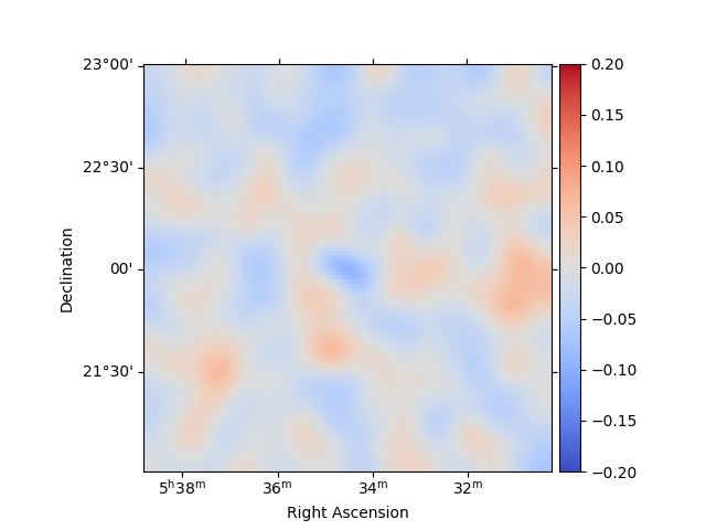
We can also directly access the .residuals() to get a map, that we
can plot interactively:
residuals = stacked.residuals(method="diff")
residuals.smooth("0.08 deg").plot_interactive(
    cmap="coolwarm", vmin=-0.2, vmax=0.2, stretch="linear", add_cbar=True
)
plt.show()
interactive(children=(SelectionSlider(continuous_update=False, description='Select energy:', layout=Layout(width='50%'), options=('1.00 TeV - 1.78 TeV', '1.78 TeV - 3.16 TeV', '3.16 TeV - 5.62 TeV', '5.62 TeV - 10.0 TeV'), style=SliderStyle(description_width='initial'), value='1.00 TeV - 1.78 TeV'), RadioButtons(description='Select stretch:', options=('linear', 'sqrt', 'log'), style=DescriptionStyle(description_width='initial'), value='linear'), Output()), _dom_classes=('widget-interact',))
Plot the fitted spectrum#
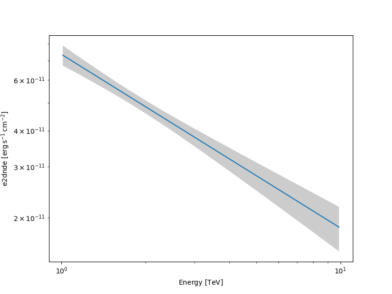
Making a butterfly plot#
The SpectralModel component can be used to produce a, so-called,
butterfly plot showing the envelope of the model taking into account
parameter uncertainties:
Now we can actually do the plot using the plot_error method:
energy_bounds = [1, 10] * u.TeV

fig, ax = plt.subplots(figsize=(8, 6))
spec.plot(ax=ax, energy_bounds=energy_bounds, sed_type="e2dnde")
spec.plot_error(ax=ax, energy_bounds=energy_bounds, sed_type="e2dnde")
plt.show()
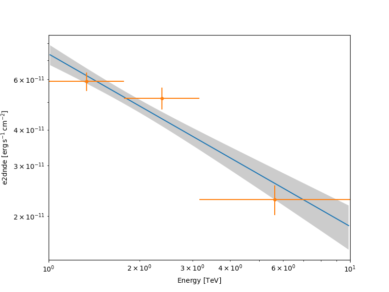
Computing flux points#
We can now compute some flux points using the
FluxPointsEstimator.
Besides the list of datasets to use, we must provide it the energy intervals on which to compute flux points as well as the model component name.
energy_edges = [1, 2, 4, 10] * u.TeV
fpe = FluxPointsEstimator(energy_edges=energy_edges, source="crab")

flux_points = fpe.run(datasets=[stacked])

fig, ax = plt.subplots(figsize=(8, 6))
spec.plot(ax=ax, energy_bounds=energy_bounds, sed_type="e2dnde")
spec.plot_error(ax=ax, energy_bounds=energy_bounds, sed_type="e2dnde")
flux_points.plot(ax=ax, sed_type="e2dnde")
plt.show()
/home/runner/work/gammapy-docs/gammapy-docs/gammapy/.tox/build_docs/lib/python3.12/site-packages/gammapy/maps/region/ndmap.py:154: UserWarning: This axis already has a converter set and is updating to a potentially incompatible converter
  ax.errorbar(