Note
Go to the end to download the full example code or to run this example in your browser via Binder.
Spectral analysis with the HLI#
Introduction to 1D analysis using the Gammapy high level interface.
Prerequisites#
Understanding the gammapy data workflow, in particular what are DL3 events and instrument response functions (IRF).
Context#
This notebook is an introduction to gammapy analysis using the high level interface.
Gammapy analysis consists of two main steps.
The first one is data reduction: user selected observations are reduced to a geometry defined by the user. It can be 1D (spectrum from a given extraction region) or 3D (with a sky projection and an energy axis). The resulting reduced data and instrument response functions (IRF) are called datasets in Gammapy.
The second step consists of setting a physical model on the datasets and fitting it to obtain relevant physical information.
Objective: Create a 1D dataset of the Crab using the H.E.S.S. DL3 data release 1 and perform a simple model fitting of the Crab nebula.
Proposed approach#
This notebook uses the high level Analysis class to orchestrate data
reduction and run the data fits. In its current state, Analysis
supports the standard analysis cases of joint or stacked 3D and 1D
analyses. It is instantiated with an AnalysisConfig object that
gives access to analysis parameters either directly or via a YAML config
file.
To see what is happening under-the-hood and to get an idea of the
internal API, a second notebook performs the same analysis without using
the Analysis class.
In summary, we have to:
Create an
AnalysisConfigobject and the analysis configuration:Define what observations to use
Define the geometry of the dataset (data and IRFs)
Define the model we want to fit on the dataset.
Instantiate a
Analysisfrom this configuration and run the different analysis stepsObservation selection
Data reduction
Model fitting
Estimating flux points
from pathlib import Path

# %matplotlib inline
import matplotlib.pyplot as plt
Setup#
from IPython.display import display
from gammapy.analysis import Analysis, AnalysisConfig
from gammapy.modeling.models import Models
Analysis configuration#
For configuration of the analysis we use the YAML data format. YAML is a machine-readable serialisation format, that is also friendly for humans to read. In this tutorial we will write the configuration file just using Python strings, but of course the file can be created and modified with any text editor of your choice.
Here is what the configuration for our analysis looks like:
yaml_str = """
observations:
    datastore: $GAMMAPY_DATA/hess-dl3-dr1
    obs_cone: {frame: icrs, lon: 83.633 deg, lat: 22.014 deg, radius: 5 deg}

datasets:
    type: 1d
    stack: true
    geom:
        axes:
            energy: {min: 0.5 TeV, max: 30 TeV, nbins: 20}
            energy_true: {min: 0.1 TeV, max: 50 TeV, nbins: 40}
    on_region: {frame: icrs, lon: 83.633 deg, lat: 22.014 deg, radius: 0.11 deg}
    containment_correction: true
    safe_mask:
       methods: ['aeff-default', 'aeff-max']
       parameters: {aeff_percent: 0.1}
    background:
        method: reflected
fit:
    fit_range: {min: 1 TeV, max: 20 TeV}

flux_points:
    energy: {min: 1 TeV, max: 20 TeV, nbins: 8}
    source: 'crab'
"""

config = AnalysisConfig.from_yaml(yaml_str)
print(config)
AnalysisConfig

    general:
        log:
            level: info
            filename: null
            filemode: null
            format: null
            datefmt: null
        outdir: .
        n_jobs: 1
        datasets_file: null
        models_file: null
    observations:
        datastore: /home/runner/work/gammapy-docs/gammapy-docs/gammapy-datasets/dev/hess-dl3-dr1
        obs_ids: []
        obs_file: null
        obs_cone:
            frame: icrs
            lon: 83.633 deg
            lat: 22.014 deg
            radius: 5.0 deg
        obs_time:
            start: null
            stop: null
        required_irf:
        - aeff
        - edisp
        - psf
        - bkg
    datasets:
        type: 1d
        stack: true
        geom:
            wcs:
                skydir:
                    frame: null
                    lon: null
                    lat: null
                binsize: 0.02 deg
                width:
                    width: 5.0 deg
                    height: 5.0 deg
                binsize_irf: 0.2 deg
            selection:
                offset_max: 2.5 deg
            axes:
                energy:
                    min: 0.5 TeV
                    max: 30.0 TeV
                    nbins: 20
                energy_true:
                    min: 0.1 TeV
                    max: 50.0 TeV
                    nbins: 40
        map_selection:
        - counts
        - exposure
        - background
        - psf
        - edisp
        background:
            method: reflected
            exclusion: null
            parameters: {}
        safe_mask:
            methods:
            - aeff-default
            - aeff-max
            parameters:
                aeff_percent: 0.1
        on_region:
            frame: icrs
            lon: 83.633 deg
            lat: 22.014 deg
            radius: 0.11 deg
        containment_correction: true
    fit:
        fit_range:
            min: 1.0 TeV
            max: 20.0 TeV
    flux_points:
        energy:
            min: 1.0 TeV
            max: 20.0 TeV
            nbins: 8
        source: crab
        parameters:
            selection_optional: all
    excess_map:
        correlation_radius: 0.1 deg
        parameters: {}
        energy_edges:
            min: null
            max: null
            nbins: null
    light_curve:
        time_intervals:
            start: null
            stop: null
        energy_edges:
            min: null
            max: null
            nbins: null
        source: source
        parameters:
            selection_optional: all
    metadata:
        creator: Gammapy 2.0.dev4000+g6ed4106cb
        date: '2026-07-21T07:41:46.388585'
        origin: null
Note that you can save this string into a yaml file and load it as follows:
# config = AnalysisConfig.read("config-1d.yaml")
# # the AnalysisConfig gives access to the various parameters used from logging to reduced dataset geometries
# print(config)
Using data stored into your computer#
Here, we want to use Crab runs from the H.E.S.S. DL3-DR1. We have defined the datastore and a cone search of observations pointing with 5 degrees of the Crab nebula. Parameters can be set directly or as a python dict.
PS: do not forget to set up your environment variable $GAMMAPY_DATA to
your local directory containing the H.E.S.S. DL3-DR1 as described in
Recommended Setup.
Setting the exclusion mask#
In order to properly adjust the background normalisation on regions
without gamma-ray signal, one needs to define an exclusion mask for the
background normalisation. For this tutorial, we use the following one
$GAMMAPY_DATA/joint-crab/exclusion/exclusion_mask_crab.fits.gz
config.datasets.background.exclusion = (
    "$GAMMAPY_DATA/joint-crab/exclusion/exclusion_mask_crab.fits.gz"
)
We’re all set. But before we go on let’s see how to save or import
AnalysisConfig objects though YAML files.
Using YAML configuration files for setting/writing the Data Reduction parameters#
One can export/import the AnalysisConfig to/from a YAML file.
config.write("config.yaml", overwrite=True)

config = AnalysisConfig.read("config.yaml")
print(config)
AnalysisConfig

    general:
        log:
            level: info
            filename: null
            filemode: null
            format: null
            datefmt: null
        outdir: .
        n_jobs: 1
        datasets_file: null
        models_file: null
    observations:
        datastore: /home/runner/work/gammapy-docs/gammapy-docs/gammapy-datasets/dev/hess-dl3-dr1
        obs_ids: []
        obs_file: null
        obs_cone:
            frame: icrs
            lon: 83.633 deg
            lat: 22.014 deg
            radius: 5.0 deg
        obs_time:
            start: null
            stop: null
        required_irf:
        - aeff
        - edisp
        - psf
        - bkg
    datasets:
        type: 1d
        stack: true
        geom:
            wcs:
                skydir:
                    frame: null
                    lon: null
                    lat: null
                binsize: 0.02 deg
                width:
                    width: 5.0 deg
                    height: 5.0 deg
                binsize_irf: 0.2 deg
            selection:
                offset_max: 2.5 deg
            axes:
                energy:
                    min: 0.5 TeV
                    max: 30.0 TeV
                    nbins: 20
                energy_true:
                    min: 0.1 TeV
                    max: 50.0 TeV
                    nbins: 40
        map_selection:
        - counts
        - exposure
        - background
        - psf
        - edisp
        background:
            method: reflected
            exclusion: /home/runner/work/gammapy-docs/gammapy-docs/gammapy-datasets/dev/joint-crab/exclusion/exclusion_mask_crab.fits.gz
            parameters: {}
        safe_mask:
            methods:
            - aeff-default
            - aeff-max
            parameters:
                aeff_percent: 0.1
        on_region:
            frame: icrs
            lon: 83.633 deg
            lat: 22.014 deg
            radius: 0.11 deg
        containment_correction: true
    fit:
        fit_range:
            min: 1.0 TeV
            max: 20.0 TeV
    flux_points:
        energy:
            min: 1.0 TeV
            max: 20.0 TeV
            nbins: 8
        source: crab
        parameters:
            selection_optional: all
    excess_map:
        correlation_radius: 0.1 deg
        parameters: {}
        energy_edges:
            min: null
            max: null
            nbins: null
    light_curve:
        time_intervals:
            start: null
            stop: null
        energy_edges:
            min: null
            max: null
            nbins: null
        source: source
        parameters:
            selection_optional: all
    metadata:
        creator: Gammapy 2.0.dev4000+g6ed4106cb
        date: '2026-07-21T07:41:46.401804'
        origin: null
Running the first step of the analysis: the Data Reduction#
Configuration of the analysis#
We first create an Analysis object from our
configuration.
Observation selection#
We can directly select and load the observations from disk using
get_observations():
The observations are now available on the Analysis object.
The selection corresponds to the following ids:
print(analysis.observations.ids)
['23523', '23526', '23559', '23592']
To see how to explore observations, please refer to the following notebook: CTAO with Gammapy or H.E.S.S. with Gammapy
Running the Data Reduction#
Now we proceed to the data reduction. In the config file we have chosen
a WCS map geometry, energy axis and decided to stack the maps. We can
run the reduction using get_datasets():
Results exploration#
As we have chosen to stack the data, one can print what contains the unique entry of the datasets:
print(analysis.datasets[0])
SpectrumDatasetOnOff
--------------------

  Name                            : stacked

  Total counts                    : 427
  Total background counts         : 25.86
  Total excess counts             : 401.14

  Predicted counts                : 43.14
  Predicted background counts     : 43.14
  Predicted excess counts         : nan

  Exposure min                    : 2.90e+07 m2 s
  Exposure max                    : 2.64e+09 m2 s

  Number of total bins            : 20
  Number of fit bins              : 18

  Fit statistic type              : wstat
  Fit statistic value (-2 log(L)) : 1396.10

  Number of models                : 0
  Number of parameters            : 0
  Number of free parameters       : 0

  Total counts_off                : 581
  Acceptance                      : 70
  Acceptance off                  : 1756
As you can see the dataset uses WStat with the background computed with the Reflected Background method during the data reduction, but no source model has been set yet.
The counts, exposure and background, etc are directly available on the dataset and can be printed:
info_table = analysis.datasets.info_table()
info_table

print(
    f"Tobs={info_table['livetime'].to('h')[0]:.1f} Excess={info_table['excess'].value[0]:.1f} \
Significance={info_table['sqrt_ts'][0]:.2f}"
)
Tobs=1.8 h Excess=401.1 Significance=37.04
Save dataset to disk#
It is common to run the preparation step independent of the likelihood fit, because often the preparation of counts, collection are and energy dispersion is slow if you have a lot of data. We first create a folder:
path = Path("hli_spectrum_analysis")
path.mkdir(exist_ok=True)
And then write the stacked dataset to disk by calling the dedicated
write() method:
filename = path / "crab-stacked-dataset.fits.gz"
analysis.datasets.write(filename, overwrite=True)
Model fitting#
Creation of the model#
First, let’s create a model to be adjusted. As we are performing a 1D
Analysis, only a spectral model is needed within the SkyModel
object. Here is a pre-defined YAML configuration file created for this
1D analysis:
model_str = """
components:
- name: crab
  type: SkyModel
  spectral:
    type: PowerLawSpectralModel
    parameters:
      - name: index
        frozen: false
        scale: 1.0
        unit: ''
        value: 2.6
      - name: amplitude
        frozen: false
        scale: 1.0
        unit: cm-2 s-1 TeV-1
        value: 5.0e-11
      - name: reference
        frozen: true
        scale: 1.0
        unit: TeV
        value: 1.0
"""
model_1d = Models.from_yaml(model_str)
print(model_1d)
Models

Component 0: SkyModel

  Name                      : crab
  Datasets names            : None
  Spectral model type       : PowerLawSpectralModel
  Spatial  model type       :
  Temporal model type       :
  Parameters:
    index                         :      2.600   +/-    0.00
    amplitude                     :   5.00e-11   +/- 0.0e+00 1 / (TeV s cm2)
    reference             (frozen):      1.000       TeV
Or from a yaml file, e.g.
# model_1d = Models.read("model-1d.yaml")
# print(model_1d)
Now we set the model on the analysis object:
Setting fitting parameters#
Analysis can perform a few modeling and fitting tasks besides data
reduction. Parameters have then to be passed to the configuration
object.
Running the fit#
Exploration of the fit results#
print(analysis.fit_result)

display(model_1d.to_parameters_table())
OptimizeResult

        backend    : minuit
        method     : migrad
        success    : True
        message    : Optimization terminated successfully.
        nfev       : 37
        total stat : 10.29

CovarianceResult

        backend    : minuit
        method     : hesse
        success    : True
        message    : Hesse terminated successfully.

model type    name     value         unit      ... min max frozen link prior
----- ---- --------- ---------- -------------- ... --- --- ------ ---- -----
 crab          index 2.6768e+00                ... nan nan  False
 crab      amplitude 4.6795e-11 TeV-1 s-1 cm-2 ... nan nan  False
 crab      reference 1.0000e+00            TeV ... nan nan   True
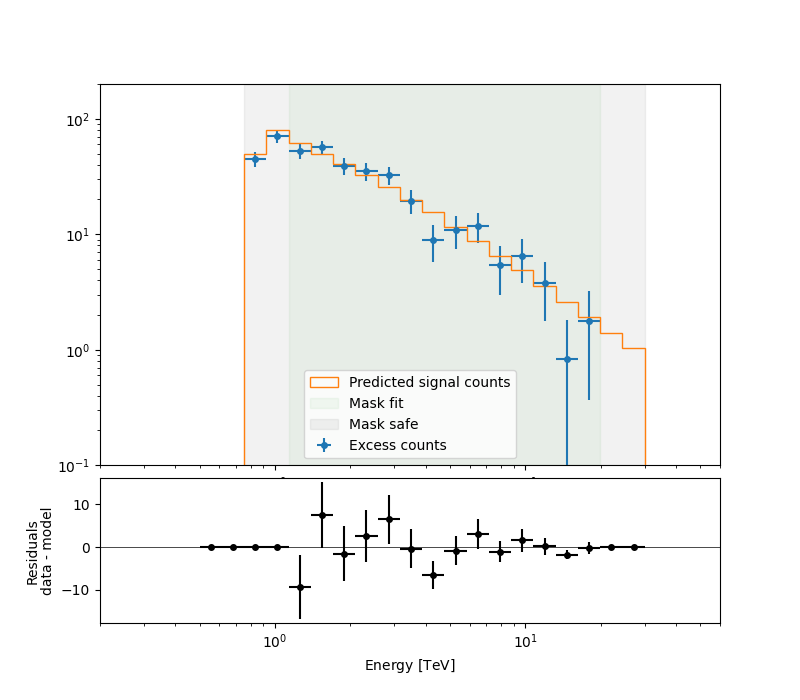
To check the fit is correct, we compute the excess spectrum with the predicted counts.
ax_spectrum, ax_residuals = analysis.datasets[0].plot_fit()
ax_spectrum.set_ylim(0.1, 200)
ax_spectrum.set_xlim(0.2, 60)
ax_residuals.set_xlim(0.2, 60)
plt.show()
Serialisation of the fit result#
This is how we can write the model back to file again:
filename = path / "model-best-fit.yaml"
analysis.models.write(filename, overwrite=True)

with filename.open("r") as f:
    print(f.read())
components:
-   name: crab
    type: SkyModel
    spectral:
        type: PowerLawSpectralModel
        parameters:
        -   name: index
            value: 2.67683698668005
            error: 0.10350022377526517
        -   name: amplitude
            value: 4.6794780053275544e-11
            unit: TeV-1 s-1 cm-2
            error: 4.6786842409412115e-12
        -   name: reference
            value: 1.0
            unit: TeV
covariance: model-best-fit_covariance.dat
metadata:
    creator: Gammapy 2.0.dev4000+g6ed4106cb
    date: '2026-07-21T07:41:48.583569'
    origin: null
Creation of the Flux points#
Running the estimation#
analysis.get_flux_points()

crab_fp = analysis.flux_points.data
crab_fp_table = crab_fp.to_table(sed_type="dnde", formatted=True)
display(crab_fp_table)
e_ref  e_min  e_max        dnde      ... is_ul counts success   norm_scan
 TeV    TeV    TeV   1 / (TeV s cm2) ...
------ ------ ------ --------------- ... ----- ------ ------- --------------
 1.134  0.924  1.392       2.835e-11 ... False   56.0    True 0.200 .. 5.000
 1.708  1.392  2.096       1.193e-11 ... False  102.0    True 0.200 .. 5.000
 2.572  2.096  3.156       4.325e-12 ... False   71.0    True 0.200 .. 5.000
 3.873  3.156  4.753       1.002e-12 ... False   31.0    True 0.200 .. 5.000
 5.833  4.753  7.158       4.655e-13 ... False   24.0    True 0.200 .. 5.000
 7.929  7.158  8.784       1.527e-13 ... False    6.0    True 0.200 .. 5.000
10.779  8.784 13.228       9.692e-14 ... False   11.0    True 0.200 .. 5.000
16.233 13.228 19.921       1.523e-14 ... False    3.0    True 0.200 .. 5.000
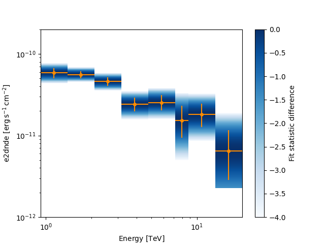
Let’s plot the flux points with their likelihood profile
fig, ax_sed = plt.subplots()
crab_fp.plot(ax=ax_sed, sed_type="e2dnde", color="darkorange")
ax_sed.set_ylim(1.0e-12, 2.0e-10)
ax_sed.set_xlim(0.5, 40)
crab_fp.plot_ts_profiles(ax=ax_sed, sed_type="e2dnde")
plt.show()
Serialisation of the results#
The flux points can be exported to a fits table following the format defined here
filename = path / "flux-points.fits"
analysis.flux_points.write(filename, overwrite=True)
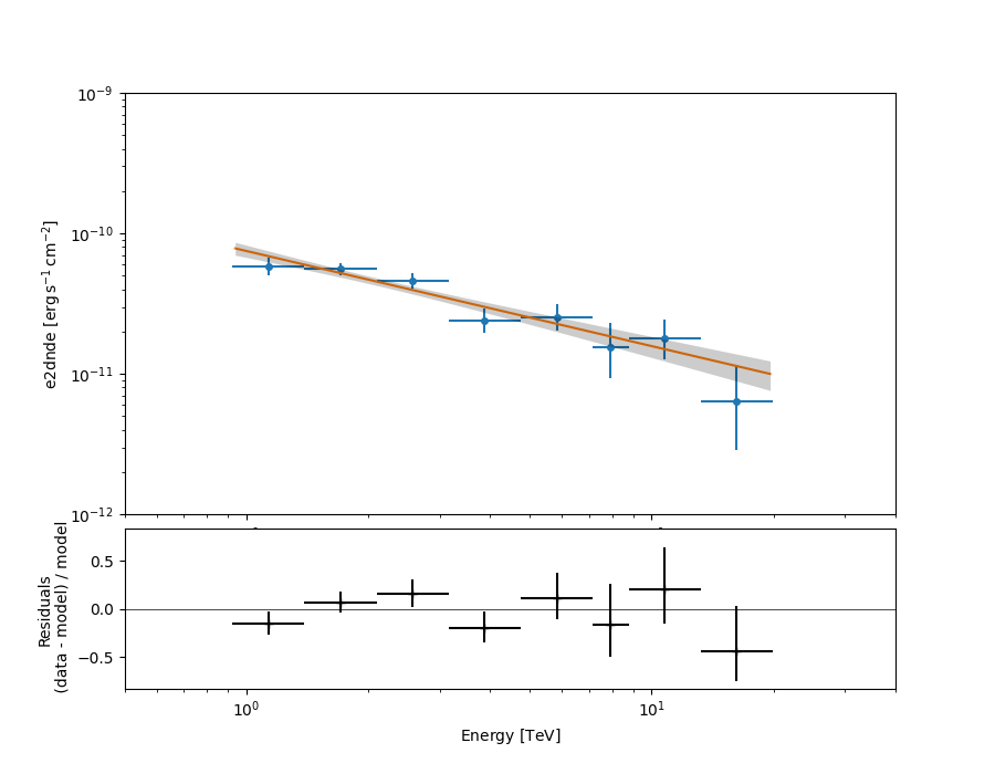
Plotting the final results of the 1D Analysis#
We can plot of the spectral fit with its error band overlaid with the flux points:
ax_sed, ax_residuals = analysis.flux_points.plot_fit()
ax_sed.set_ylim(1.0e-12, 1.0e-9)
ax_sed.set_xlim(0.5, 40)
plt.show()
/home/runner/work/gammapy-docs/gammapy-docs/gammapy/.tox/build_docs/lib/python3.12/site-packages/gammapy/modeling/models/spectral.py:649: UserWarning: This axis already has a converter set and is updating to a potentially incompatible converter
  ax.plot(energy.center, flux.quantity[:, 0, 0], **kwargs)
What’s next?#
You can look at the same analysis without the high level interface in Spectral analysis.
As we can store the best model fit, you can overlay the fit results of both methods on a unique plot.
Total running time of the script: (0 minutes 12.612 seconds)